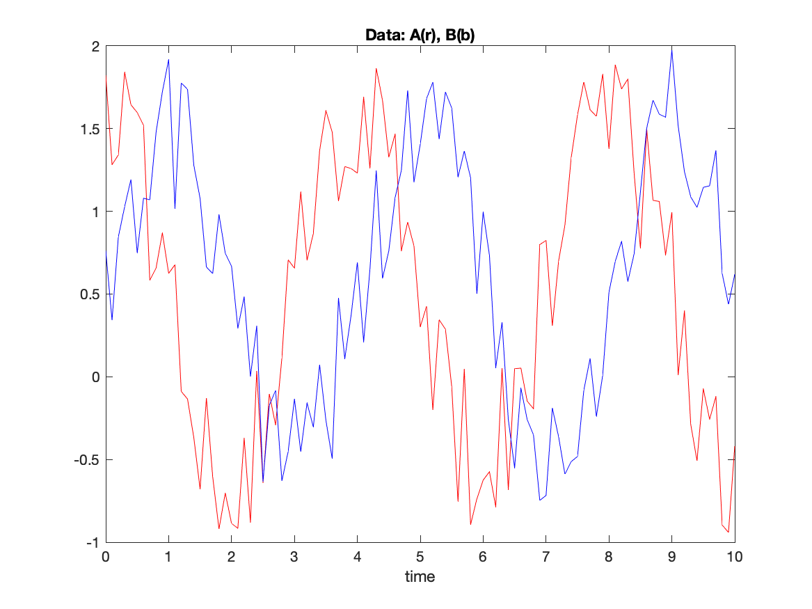
Task: What is the time shift between the two time series in the C7.dat data file. The first column is time (days) while the second and third columns are measurements of two quantities at the same location and time. Write a script to read the data file and calculate the lagged correlation between the two vectors. In a two panel plot, plot the two time series in one panel and the lagged correlation in the other. Write the time shift on the data panel.
The previous task considered the correlation between two time series. In the plot of the two vectors, you likely noticed that there were oscillations in each series. Furthermore, the peaks in the two series did not occur at the same time. You might assume that the oscillations are related and you might want to know the delay between the peaks in one series compared to another.
The hard way to do this is to plot the two time series in different plots, print each plot and shift the plots side to side until the peaks line up and read the time shift from the x axis of the plots. You could use a light table (ask an old person what this is) or you could put the plots against a window.
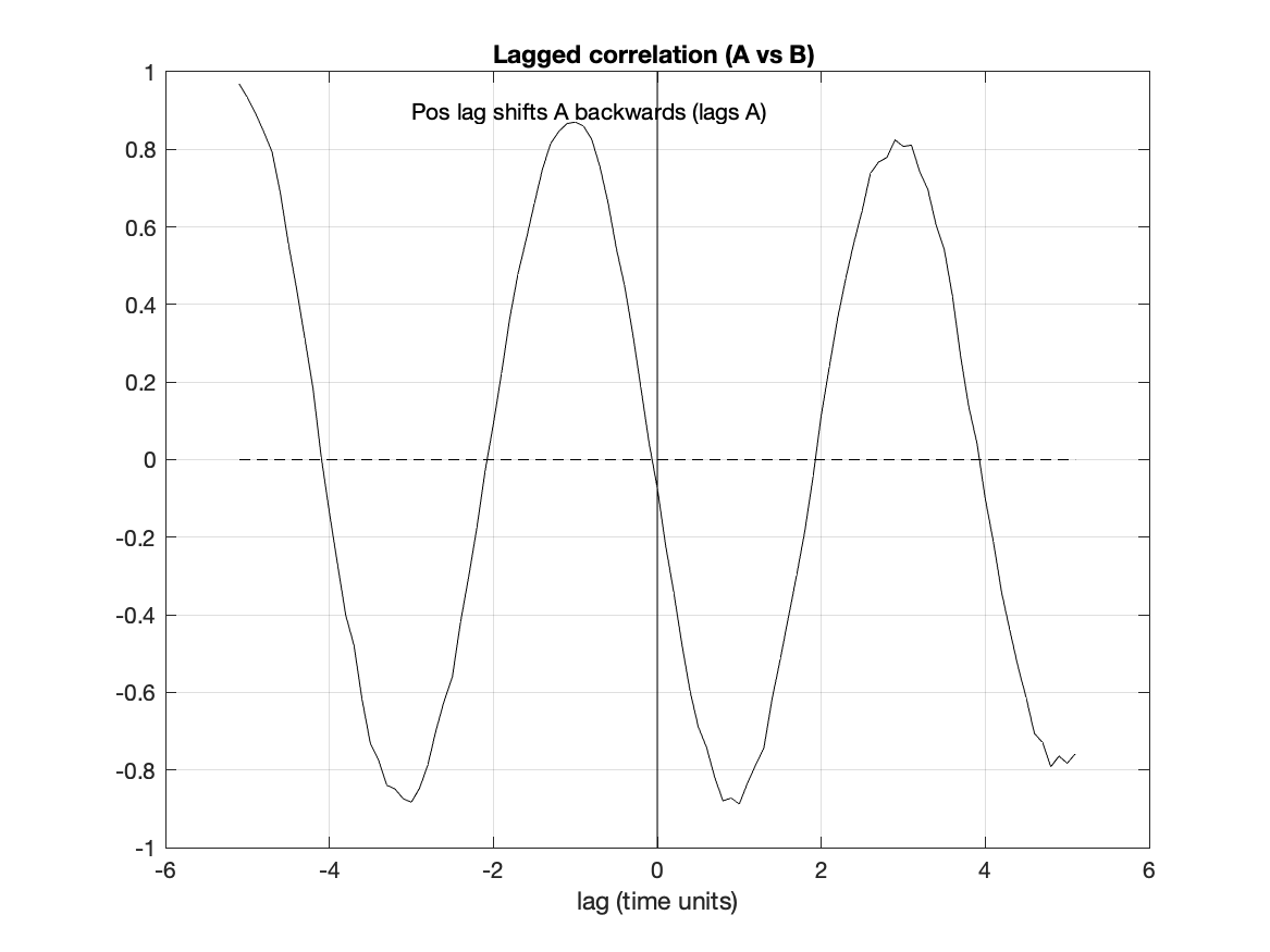
A more direct way to find the time shift is to calculate the correlation between the time series after shifting one series relative to another, referred to as a "lagged correlation".
Imagine two time series, A and B, each with N values. In the previous task, we used C=corr(A,B); to find the correlation between these two series. We can calculate a lagged correlation with the command
  cp1=corr(A(2:N),B(1:(N-1)));
  cp2=corr(A(3:N),B(1:(N-2));
  cn1=corr(A(1:(N-1)),B(2:N));
  cn2=corr(A(1:(N-2)),B(3:N));

%    and so on...
In the first line, the second value of A is lined up with the first value of B, which we interpret as a positive lag (or shift) of 1. The second line shifts the third value of A to line up with the first value of B, a lag of 2. The third and fourth commands shift the series the other direction (negative lags) by 1 and 2 places. Notice that the larger the shift, the fewer values are used in the correlation (meaning that the precision of the correlation becomes worse with increasing lag, either positive or negative).
With a little thought, you could come up with a pattern (an algorithm using for loops) that you could use to calculate the correlation for a whole series of shifts (both positive and negative).
The command [cxy lag]=xcorr(A,B); does all of this for you (almost). The command does not remove the mean from the input series nor does it normalize the result. The proper procedure is as follows:
% dt is the time interval of the data (assumed to be constant)
  dt=time(2)-time(1);
  Am=mean(A);Bm=mean(B);N=length(A); % B is same length as A
  As=std(A);Bs=std(B);
  Aa=(A-Am)/As;Ba=(B-Bm)/Bs;  %  anomaly from mean and normalize
  maxlag=round(N/2); % largest shift is by half the record length
  [cAB lag]=xcorr(Aa,Ba,maxlag,'unbiased');
  plot(lag*dt,cAB)
  title('Lagged correlation')
  xlabel('lag (time units)')
The default action of xcorr is to correlate the two series with both
forward and backward shifts.
The option unbiased says to divide the sum by the
number of values in the sum (N-abs(lag)).
The option biased says to divide the sum by the
total number of values in the input series (N).
The lag of the largest positive correlation gives the time shift needed to line up the two time series. If the lag is positive then the second series peak happens after the first series. A negative lag means that the first series peaks before the second.
Note that this is the convention used in xcorr, but there is no standard convention. Other software may shift the time series in the opposite way for a positive lag. Don't trust the documentation. Decide on a clear test case when you use new software. (What two artificial time series would make a good test case? Think about it!)
Newer versions of MATLAB have a function xcov which removes the mean from the input time series before calculating the correlation. It does not seem to divide by the standard deviation. I have not used this function, but it is available if you want to see how it works.
Flow chart to solve the task:
%%%  load data from file
%%%  separate variables
%%%  scale the time series
%%%  calculate the lagged correlation
%%%  plot the time series on one panel
%%%  add title and labels
%%%  plot the lagged correlation on the second panel
%%%  add title and labels
%%%  determine the best lag between the time series
%%%  write the lag on the data panel
Script to solve the task:
%%%  load data from file
  data=load('C7.dat)
%%%  separate variables
  time=data(:,1);A=data(:,2);B=data(:,3);
%%%  scale the time series
   As=(A-mean(A))./std(A);Bs=(B-mean(B))./std(B);
%%%  calculate the lagged correlation
  [Cab,lag]=xcorr(A,B,'unbiased');
%%%  plot the time series on one panel
  figure
    subplot(1,2,1)
     plot(time,A,'k-',time,B,'k--')
%%%  add title and labels
     title('Data: A(-), B(--)')
     xlabel('time(days)')
     ylabel('values')
%%%  plot the lagged correlation on the second panel
    subplot(1,2,2)
     plot(lag,Cab)
%%%  add title and labels
     title('Lagged correlation of A and B')
     xlabel('lag (days)')
     ylabel('Correlation')
%%%  determine the best lag between the time series
%    The largest correlation is at a lag of -3 days
%     The peak of A occurs about three days before the peak of B
%%%  write the lag on the data panel
     text(6,.8,'A peaks 3 days before B peaks')