Task: Write a script to read the data file from task 5.1, extract time and D1 (second column). Calculate the variance of D1. Fit a linear, quadratic and cubic polynomial to D1. In a 4 panel figure, plot the original data and the 3 different fits (one in each panel). In the fourth panel, plot (use semilog scaling) the residual from each fit (using different colors). For each of these fitted curves, calculate the fraction of variance explained. How well does each curve represent the data?
The function polyfit returns diagnostics of the functional fit; you can find the details with help polyfit or doc polyfit. It is sometimes more useful to do your own analysis of the quality of the fit.
A measure of the quality of the fit is the size of the difference between the original data points (x(t)) and the reconstructed values from the fitted curve (xf(t)), termed the residual. The code fragment below shows the various calculations.
  varX=var(x);
  a1=polyfit(t,x,1); % linear fit
  xf=polyval(a1,t); % polynomial fit at data times
  E1=x-xf;          % mis-fit (errror) between data and linear polynomial.
  varE1=var(E1);
  VarExplained= (varX-varE1)/varX; % fraction of original variance explained
The trailing number in the variable names indicated the order of the polynomial that was used in the fit.
If the polynomial is a perfect fit, then the difference between the data and the fit will be zero for all values, so the variance of the error will be zero. Therefore, the variance explained will be 1.0 (100%).
It is useful sometimes to fit a series of polynomials of increasing order and look for a minimum in variance explained. It is also useful to look at a plot of the residual which could indicate a different functional form to fit. The best outcome is to find that the residual is random with a normal (gaussian) distribution. We will not pursue this detailed analysis at this time.
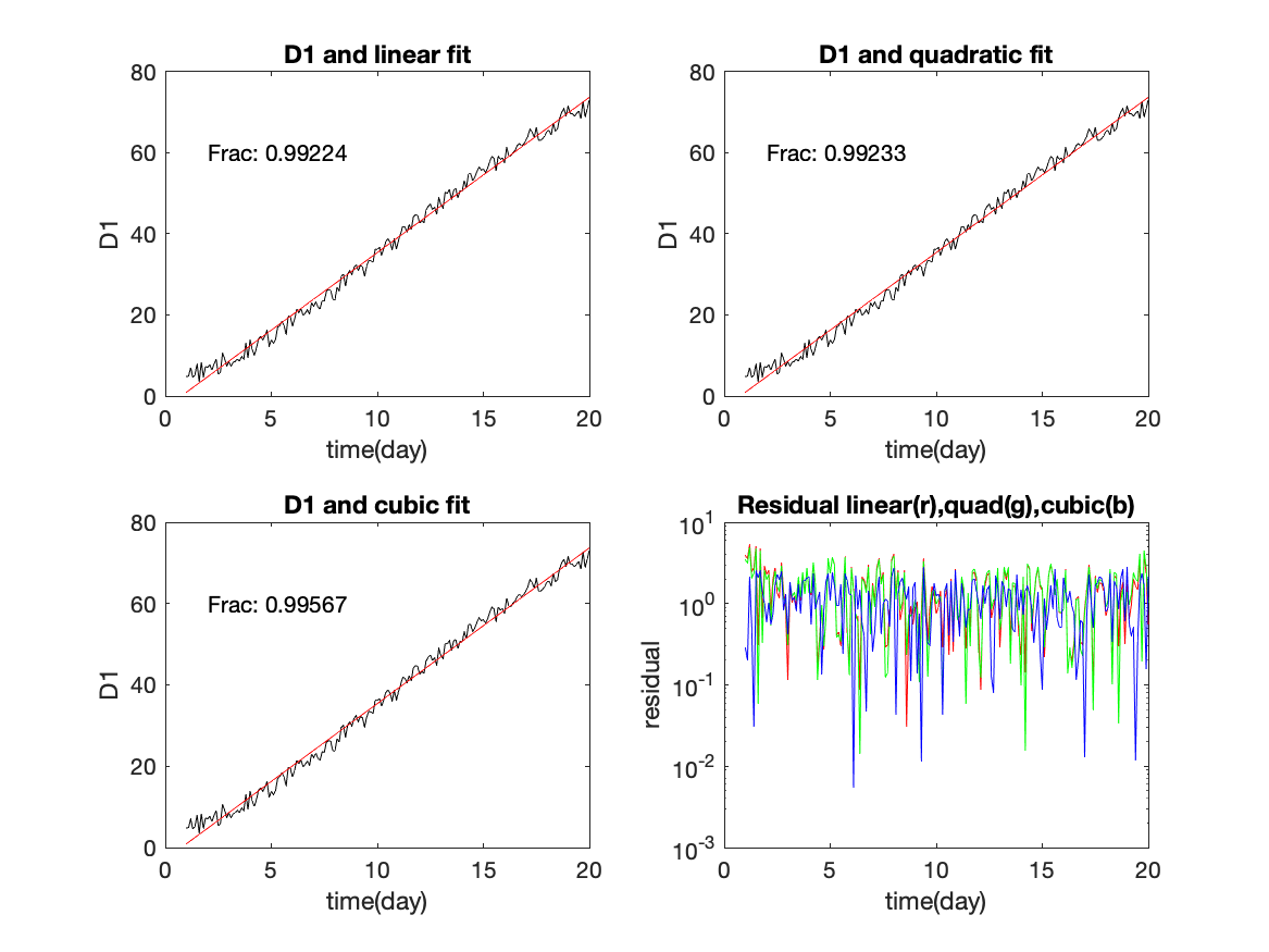
Here is the figure responding to this task. Note that over 99% of the variance is explained by all three fits. There is very little difference in the quality of these fits, although higher order polynomials have a bit better fit.
The original variance is very large for this case because of the strong trend in time. It would be more informative to calculate the variance after removing a linear trend. Then the benefit of the quadratic or cubic fit would be more obvious.
Flow chart for task 5.6
%%%  Task 5.6
%%%  read data, extract variables
%%%  fit polynomials of order 1, 2, 3 to d1
%%%  calculate the fit polynomial at data points
%%%  calculate variance of original data
%%%  calculate variance of difference between data and fit
%%%  set up subplots
%%%  for each order polynomial
%%%     plot original data and fit
%%%     write variance explained on plot
%%%     add title and legends
%%%  plot error misfit for each order on a semilog plot
%%%  add title and legends
Here is the script to generate the answer to this task.
%%%  Task 5.6
%%%  read data, extract variables
  data=load('fitdata.dat');
  time=data(:,1);D1=data(:,2);
%%%  fit polynomials of order 1, 2, 3 to d1
%%%  calculate the fit polynomial at data points
  p1=polyfit(time,D1,1);D11=polyval(p1,time);
  p2=polyfit(time,D1,2);D12=polyval(p2,time);
  p3=polyfit(time,D1,3);D13=polyval(p3,time);
%%%  calculate variance of original data
%%%  calculate variance of difference between data and fit
  vD1=var(D1);vD11=var(D11-D1);
  vD12=var(D12-D1);vD13=var(D13-D1);
  FV1=(vD1-vD11)/vD1;FV2=(vD1-vD12)/vD1;  FV3=(vD1-vD13)/vD1;
%%%  set up subplots
  figure
%%%  for each order polynomial (linear)
%%%     plot original data and fit
%%%     write variance explained on plot
   subplot(2,2,1)
    plot(time,D1,'k',time,D11,'r')
%%%     write variance explained on plot
    text(2,60,['Frac: ',num2str(FV1)])
%%%     add title and legends
    title('D1 and linear fit')
    xlabel('time(day)')
    ylabel('D1')
%%%  for each order polynomial (second)
%%%     plot original data and fit
%%%     write variance explained on plot
   subplot(2,2,2)
    plot(time,D1,'k',time,D11,'r')
%%%     write variance explained on plot
    text(2,60,['Frac: ',num2str(FV2)])
%%%     add title and legends
    title('D1 and quadratic fit')
    xlabel('time(day)')
    ylabel('D1')
%%%  for each order polynomial (third)
%%%     plot original data and fit
%%%     write variance explained on plot
   subplot(2,2,3)
    plot(time,D1,'k',time,D11,'r')
%%%     write variance explained on plot
    text(2,60,['Frac: ',num2str(FV3)])
%%%     add title and legends
    title('D1 and cubic fit')
    xlabel('time(day)')
    ylabel('D1')
%%%   plot error misfit for each order on a semilog plot
   subplot(2,2,4)
     semilogy(time,abs(D11-D1),'r',time,abs(D12-D1),'g',time,abs(D13-D1),'b')
%%%   add title and legends
     title('Residual linear(r),quad(g),cubic(b)')
     xlabel('time(day)')
     ylabel('residual')