
Task: Smooth a set of 2 dimensional observations (a table of numbers) in S7.dat to remove small scale random variations. The numbers are a set of (21x21) values which can be read into an array with the load command. First smooth 1 dimensional data by selecting the numbers in column 6 of the array. Then smooth the whole 2D array. In both cases, plot the original and smoothed values.
Small scale variations appear in almost all measurements or results from numerical calculations; we call this variability "noise". There are many sources for this variability, which is beyond the scope of the discussion here. The main concern is how to reduce the magnitude of the noise in the numerical calculations or observations that we work with.
We start with a discussion of noise in a list of numbers, for example, a series of measurements at one place over time (a time series). The character of noise is that it is not correlated (have no relationship) from one measurement to the next and that its magnitude is random (most often normal or Gaussian). Because of this characteristic, noise can be reduced by some sort of averaging of adjacent values.
This leads to a techical discussion of filtering which we will consider later, but for now, we think of smoothing as a weighted average of several contiguous values. One weighting scheme is to evenly weight a sequence of values; referred to as a "boxcar" average, or a running mean.
The MATLAB function smooth does such a boxcar average on an input vector,
  xs = smooth(x);  % uses default choices (below)
  xs = smooth(x,span,method); % controls smoothing size/method
span refers to the number of values that are averaged (needs to be odd), and method is the name of one of six possible smoothing methods. By default span=5 and method='moving'. More details are given in help smooth.
Note that the function smooth is in the curve fitting toolbox. Be sure to download this toolbox if you want to use this routine.
Examples of smoothed 1D curves.
The boxcar filter with span=5 will replace the kth value with
xs(k) = (x(k-2)+x(k-1)+x(k)+x(k+1)+x(k+2))/5;If x is a time series of some sort, then both past and future values are used in the smoothing.
The boxcar filter is not a particularly good way to filter as it can amplify certain periodic oscillations in the input series. We will not worry too much about these details for the moment and just use it as a "quick-and-dirty" smoother. The "robust Lowess" filter is recommended if there are outliers in the input data.
Another issue is the use of "future" values in the filter. If one is smoothing spatial data (say elevations along a line), then this is not such an issue. But if the measurements are over time, then it might violate causality to use future values in an average. Just think about it, and decide if this is an issue in the analysis you are doing.
Another simple filter is the 1-2-1 filter which completely removes alternating noise; that is, noise that is a positive excursion at one point, followed by a negative excursion at the next point, followed by a positive excursion at the next and so on. The 1-2-1 in the name refers to the weights in a 3 point filter.
The following code implements the filter on a vector x.
  %  read x from a file
  xs=zeros(size(x));n=length(x);
%   smooth all but the first and last points
  xs(2:(n-1))= (x(1:(n-2)) + 2*x(2:(n-1)) + x(3:n))/4;
%   smooth the first point
  xs(1)=(x(1)+x(2))/2;
%   smooth the last point
  xs(n)=(x(n-1)+x(n))/2;
The smoothing at the beginning and end of the vector assumes that the slope of the data at the ends is zero. That is, x(0)=x(2) and x(n+1)=x(n-1). The values x(0) and x(n+1) are not in the original data and are considered "ghost points" or "data extensions". They are phony values which are given some convenient value based on some assumption.
Similar techniques are used to filter in 2 dimension. One idea is to smooth with a weighted average in one direction and then smooth with the same weighted average in the other direction. This will work, but it is not always a good idea. A better technique is to use a 2D filter that sweeps through the data, similar to the 1D smoother above.
The function filter2 does such an operation, but it requires the user to enter the weights used in the average. The following code is an extention of the default smoothing operation in smooth, using a 5 point boxcar in two directions.
  %     create a 5x5 array of 1's divided by total number of points.
  W5=ones(5,5)/25;
  As5 = filter2(W5,A);  % where A is a 2D array.
As an alternative, you can create a 2D version of the 1-2-1 filter with
  W121=[1 2 1; 2 4 2; 1 2 1]/16; % 2D 1-2-1 filter (3x3)
  As121 = filter2(W121,A); % where A is a 2D array.
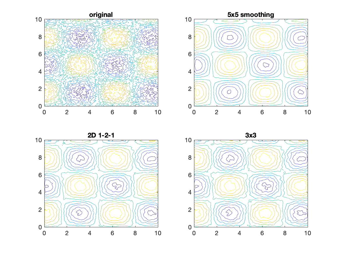
The script to create the figure above is
  x=0:.1:10;y=0:.1:10;[xA yA]=meshgrid(x,y);
  A = cos(xA).*sin(yA) + .3*rand(size(xA));
  W3=ones(3,3)/9;
  W5=ones(5,5)/25;
  W121=[1 2 1; 2 4 2; 1 2 1]/16; % 2D 1-2-1 filter (3x3)
  A5 = filter2(W5,A);
  A3 = filter2(W3,A);
  A121 = filter2(W121,A);
  figure
    subplot(2,2,1)
     contour(xA,yA,A)
     title('original')
    subplot(2,2,2)
     contour(xA,yA,A5)
     title('5x5 smoothing')
    subplot(2,2,3)
     contour(xA,yA,A3)
     title('2D 1-2-1')
    subplot(2,2,4)
     contour(xA,yA,A121)
     title('3x3')
Either of these 2D smoothing methods will reduce the small scale noise in
most arrays of numbers. Unlike smooth, filter2
assumes that you will
create the appropriate weights for the smoothing you want. So there are no
other options in this command.
Flow chart to accomplish the task:
%%%  load the array
%%%  extract column 6
%%%  smooth the 1D values
%%%  plot the original and smoothed 1D values
%%%  add legends and title
%%%  smooth the 2D values
%%%  plot the original and smoothed 2D values
%%%  add legends and title
Script to accomplish the task:
%%%  load the array
  A=load('S7.dat');
  [nr nc]=size(A);
%%%  extract column 6
  A6=A(:,6);
%%%  smooth the 1D values
  A6s=smooth(A6);
%%%  plot the original and smoothed 1D values
  figure
   x=1:nr;
   plot(x,A6,'k--',x,A6s,'r-')
%%%  add legends and title
   title('Original (k--) and smoothed (r-) data from column 6')
   xlabel('index')
   ylabel('Column 6 values')
%%%  smooth the 2D values
  W121=[1 2 1; 2 4 2; 1 2 1]/16; % 2D 1-2-1 filter (3x3)
  As121 = filter2(W121,A);
%%%  plot the original and smoothed 2D values
  figure
    subplot(1,2,1)
     contour(A)
%%%  add legends and title
     title('Original array')
    subplot(1,2,2)
     contour(As121)
%%%  add legends and title
     title('Smoothed array')