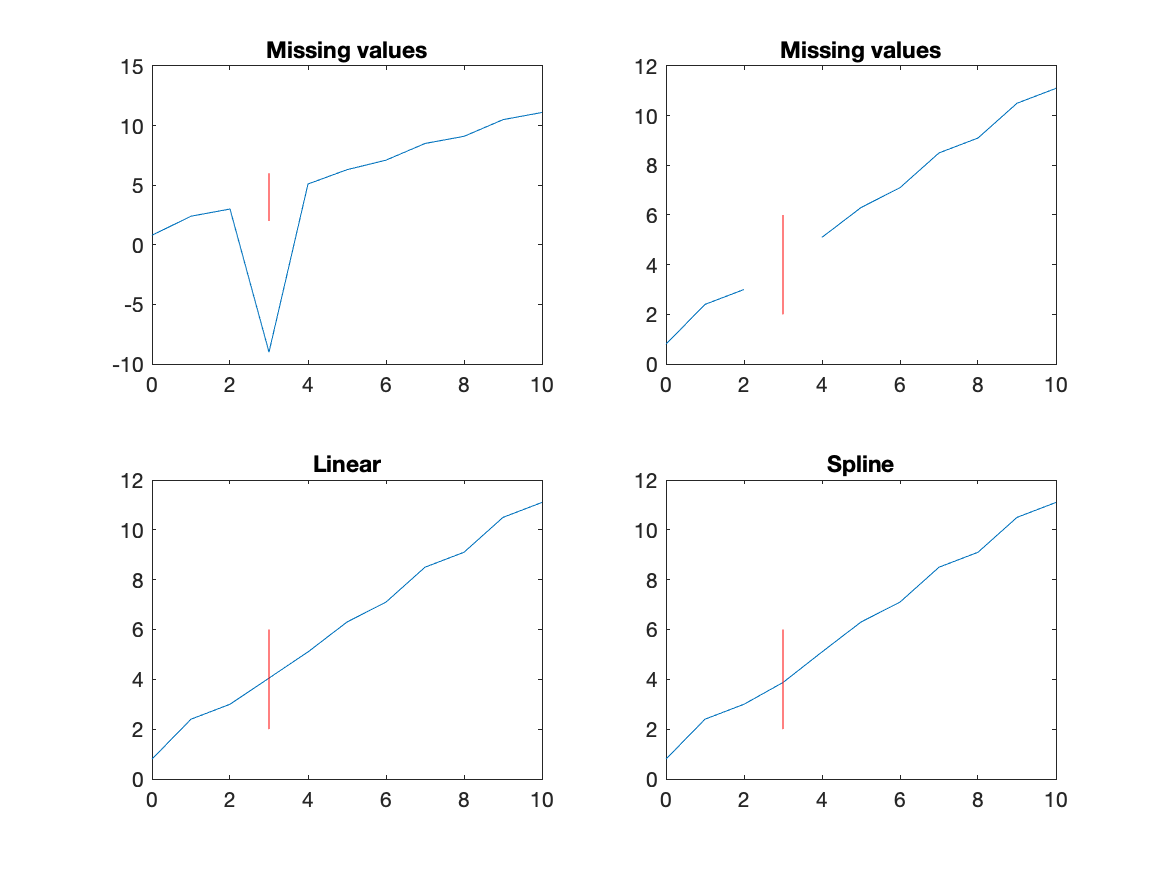
Task: Replace the missing values in this file data6.dat by interpolation. The file has a single list of numbers. Missing values are indicated by a value of -9.
Interpolation is the process of estimating a value between two or more other values. Consider two measurements with values of 3 and 5 at times 0 and 1. What is a reasonable guess at the value for time 0.5? One guess would be the average of 3 and 5, or (3+5)/2=4.
This guess is produced by fitting a straight line between the two values and evaluating the line at t=0.5. This is an example of linear interpolation.
There are other interpolation methods. One could simply choose the closest value (the value of x whose t value is closest the desired t) as the interpolated value; this is called "nearest neighbor" interpolation.
Sometimes we want to include information about the curvature of a line through the values near the interpolation point. We can do this by using two known values on either side of the location where we want an estimated value (4 values total) and fit a cubic polynomial to the four points. Then evaluate the polynomial at the location where we want the estimated value.
Each of these methods has both positive and negative characteristics.
Matlab has a function (interp1) which does interpolation in one dimension to desired points given a set of locations and values. Specifically, let x be a list of values known at times t. We desire interpolated values (xi) at another set of times (ti). Then,
xi=interp1(t,x,ti);creates the list of values that we want. This function assumes that the first array is the location or time of values provided in the second array. More generally, assume that the first array is the input and the second array is the output (result). For example, the result could be algal growth rate at different temperatures (input).
By default, this command uses linear interpolation. You can add a fourth argument to specify one of 8 interpolation methods. Cubic spline interpolation is chosen with
xi=interp1(t,x,ti,'spline');See help interp1 to get details of other options.
If the time at which we want an interpolated value is not within the range of times in the input time series, then interp1 will return NaN. That is, this function will not extrapolate outside of the range of input (t) values given.
It is possible to force extrapolation with the option 'extrap',
xi=interp1(t,x,ti,'spline','extrap');This works with any interpolation method.
There are a number of uses for interpolation in dealing with observations. One use is to estimate missing values. Another use is to convert measurements taken at random times (or input locations) to values on a time base with a uniform interval.
While easy to do, both of these choices can lead to problems. Suppose there are a large string of successive missing values. Suppose a sensor measuring water temperature every 15 minutes was not working for a month. Is it really a good idea to use interpolation to fill in the missing values? Using interpolation to replace an isolated missing measurement is likely ok, but after a long enough gap, interpolation is not a good idea.
To accomplish this interpolation, consider the following where missing values are indicated by NaN.
%   read t and x from a file
%   with -9 as the missing value
%  ig=find(x > -9);  %  get index of good (non-missing) values
%    with NaN as the missing value
  ig=find(~isnan(x));  %  get index of good (non-missing) values
  xgood = interp1(t(ig),x(ig),t);
The index ig picks the values that are ok, then interpolation estimates values at the original times, providing a new vector of values (xgood) with the same length as the original data (x). Notice that interpolation to a time that has a value, simply returns the original value.
It is important that the first and last values are good; that is, not NaN.
In the second case, suppose we want to estimate values at the beginning of every hour with a sensor measuring water temperature every 15 minutes. In this case, interpolation will likely be useful.
Suppose we have a set of measurements (e.g., air temperature) that are measured once a day within an hour of noon but not always at noon. We can create a reasonable set of measurements at fixed times as follows:
%      read a years worth of day and airtemp from a file
  iYearDay=(0:1:364)+.5;   %  create a time base for midday
  IntAirTemp=interp1(yearday,airtemp,iYearDay,'spline');
  figure
   plot(yearday,airtemp,'b',iYearDay,IntAirTemp,'r')
   title('Air Temp: orig (b), interp (r)')
It is always a good idea to plot the original and interpolated values to
make sure things worked the way you wanted.
Flow chart to solve task
%%%  read data, separate columns
%%%  identify good values
%%%  interpolate to replace bad values
Script to complete task:
%%%  read data
  data = load('data6.dat');
  n=length(data);
  t=1:n;
%%%  identify good values
  good = find(data > -9);
%%%  interpolate to replace bad values
  idata=interp1(t(good),data(good),t);
  figure
   plot(t,idata)
   title('Fixed data')