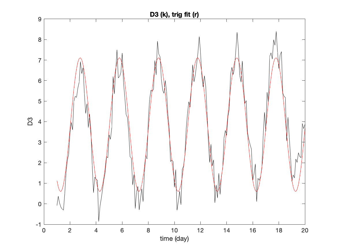
Task: Write a script to read the data file introduced in task 5.1. Extract the first (time) and fourth columns (D3) of the data matrix. Fit trigonometric functions with a period of 3 days to these values. Plot the original data vs time along with the trig function.
There is a technique to fit data to functional forms that are "linear in the coefficients". That is, if the missing coefficients multiply some function but are not "inside" the function (the example below will make this clear).
Many environmental measurements have seasonal cycles, such as we saw with the Norfolk air temperatures. In general, these have the form of sine and cosine functions of annual and semi-annual periods.
We can fit data to an oscillatory function of the form:
x(t) = a + b * cos(2*pi*t/T) + c * sin(2*pi*t/T)where T is the period of interest. This would be 365 days if we were looking for an annual cycle in daily data.
If we know the period that we are looking for, then T is not an unknown parameter; we are looking for a, b and c which are linear in the expression above.
We can fit this function to data by first constructing a "response matrix", R of the form
   T=365;
   R = [ ones(size(t)) cos(2*pi*t/T) sin(2*pi*t/T)];
where t is the time for the observations (in units of days, in this case). In addition, t must be a column vector so that the response matrix has three columns.
Given the response matrix, the fit coefficients are obtained with
  CF = R\x;
  a=CF(1);   % reconstruct coefficients
  b=CF(2);
  c=CF(3);
  xf=R*CF;   % reconstruct the fitted function
  e=x-xf;    % error of the fit
where the backslash (\) is the "left matrix divide" which translates to "matrix inverse of R matrix multiplied by x". CF is a vector with 3 numbers: the fit coefficients.
This fitting method is very general and can be used for polynomial fits. Construct a response matrix of the form:
  R = [ones(size(t)) t.^1  t.^2];
  p2=R\x;  %  calculates a quadratic polynomial fit
It is possible to add linear trends in the trigonometric fit by using a response matrix of the form:
   T=365;
   R = [ ones(size(t)) t cos(2*pi*t/T) sin(2*pi*t/T)];
which will fit data to a function of the form
x(t) = a + b*t + c*cos(2*pi*t/T) + d*sin(2*pi*t/T)which is a seasonal cycle with a trend.
It is sometimes necessary to allow for both an annual and semi-annual variations in environmenal measurements to properly represent seasonal patterns. In this case, the response matrix is
   T=365;
   R = [ones(size(t)) cos(2*pi*t/T) sin(2*pi*t/T) cos(4*pi*t/T) sin(4*pi*t/T)];
where the last two terms have two cycles per year (or a period of T/2).
Flow chart for task 5.5
%%%  Task 5.5
%%%  read data, extract variables
%%%  create response matrix
%%%  calculate fit coefficients
%%%  reconstruct polynomial from fit
%%%  plot original data and fit curve
%%%  add legends and title
Here is the script to generate the answer to this task.
%%%  Task 5.5
%%%  read data, extract variables
  data=load('fitdata.dat');
  time=data(:,1);D3=data(:,4);
%%%  create response matrix
  R=[ones(size(time)) cos(2*pi*time/3) sin(2*pi*time/3)];
%%%  calculate fit coefficients
  CF=R\D3;
%%%  reconstruct polynomial from fit
  D3f=R*CF;
%%%  plot original data and fit curve
  figure
    plot(time,D3,'k',time,D3f,'r')
%%%  add legends and title
    title('D3 (k), trig fit (r)')
    xlabel('time (day)')
    ylabel('D3')
Here is the figure responding to this task.