Task: Given exponential growth of a population with a rate of 0.1 per year, use a numerical solution to determine the number of years required for the population to increase by a factor of 5. Write a script to solve the exponential growth ODE. Start with an initial population of 10. Plot both the numerical and analytical solution on the same graph.
Calculus is the mathematics of change. An ordinary differential equation (ODE) is a statement of the rate that some variable changes based on the values of the variable or time. Typically, a first order equation has the form:
dX/dt = F(X,t)where F is some function. A math class about ODE teaches you how to solve these equations for specific forms of the right hand side (RHS) of this equation. First-order refers to the fact that the equation involves at most a first derivative of the dependent variable (X, in this case).
T.R. Maltus wrote in 1798 that human population increases in proportion to the number of people in the population (exponential growth) while food increases at a constant rate (linear growth). He forecast that there would be a population crisis as the number of people outgrew their capacity to grow food.
His idea is specified with the first order ODE
dP/dt = g * Pwhere P [number] is the number of people and g [fraction/year] or [young people per reproducing people per year) is the net expansion rate of the population (rate that new people enter the population per time interval).
This equation is easy to solve analytically, with the added condition that the initial population is Po
P(t) = Po * exp( g * t)which is the classic exponential (unconstrained) expansion of a population. These models apply to biological, chemical and radioactive systems of all sorts, not just human populations.
It is possible to solve these equations numerically. The RHS of the equation above is just the slope of the line at some time and some population level. It is possible to use the slope to step a bit into the future to estimate a new value for X. One way to do this is
  NewValue = CurrentValue +  TimeInterval * CurrentSlope
  X(t+dt) = X(t) +  dt * F(X(t), t)
where dt is a short time interval.
Actually, this is not a very good solution method. There are a number of better, but more complicated, ways to numerically solve an ODE.
Luckily, MATLAB has several tools for calculating the numerical solution to a first order ODE, one of which is ODE45. We will use this solver without worrying about how or why it works (although I can talk about it after class if you are interested).
The solver routine requires 3 bits of information to work. The first argument is the name of the function that defines the right-hand side of the ODE to be solved. This function will be given the current time and the current value of the variables and asked to provide the time change of each variable (basically, the evaluation of the right-hand side (RHS) of the ODE.
The character @ in front of the function name indicates that the name of the function is being provided. Without this leading symbol, MATLAB will evaluate the function and pass a set of values (which is not what is needed.
The second argument is the time span for the simulation. It contains two values: the start and finish time. The solution will cover this time span, but not with a uniform time interval.
The third argument is the initial value for each of the variables in the model.
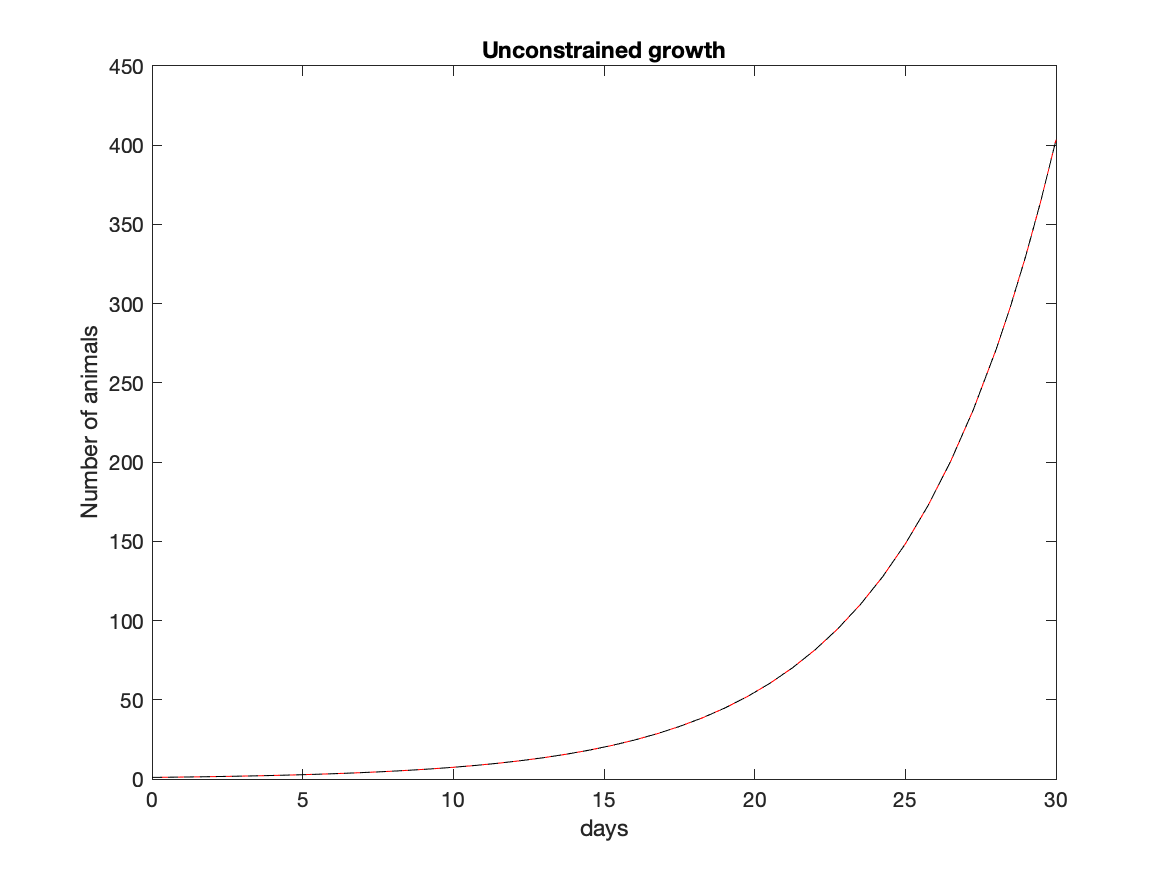
We can test ode45 with the Malthus model as follows. We define a function (called Malthus) to calculate the slope (dP/dt). Then the script below sets the values and calls the solver storing the times (t) and populations (P) obtained by the calculation.
%  MalthusODE
%  test the ode solver using Malthus to define dPdt = g * P
%
global g
g=.1;
tspan=[0 10];  % time span for the solution.
Po=10;   %  Initial population (in  thousands)
[t P]=ode45(@Malthus, tspan, Po);   % solve the equation
TrueP=Po*exp(g*t);
figure
  plot(t,P,'r',t,TrueP,'k--')
function dPdt  = Malthus(t,P)
% dPdt is uncontrained growth
global g
  dPdt = g * P;
end
The growth rate is specified by g and the initial population is specified by Po. The variable tspan gives the beginning and ending times for the solution. The solver will decide internally how often to calculate the solution (that is, how big dt is). The script calculates the true solution to plot along with the numerical solution.
A more reasonable model allows the population to both grow and die. In that case, the model equation looks like
dP/dt = g * P - m * P = (g - m)*PWe can determine the steady population by finding the population level at which the population does not change or dP/dt = 0.
For the constant growth and mortality model, the steady state condition is
(g - m) * P = 0which is zero only if g = m. That is, the growth rate of the population matches the death rate.
This is not an interesting answer. Thinking a bit, we realize that growth depends on the population, but the mortality rate should increase with the population, because food will become a limitation (or diseases are easier to spread, or any number of other reasons). In this case the model becomes
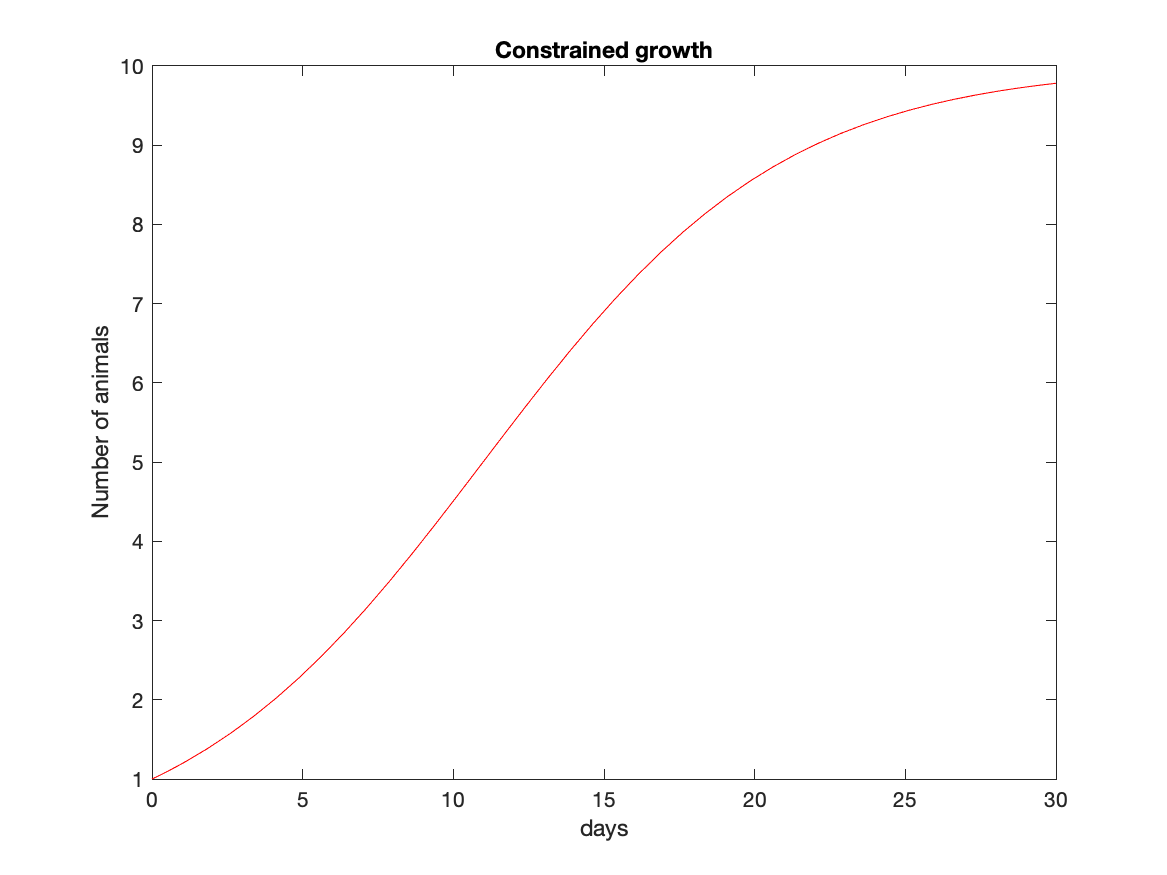
dP/dt = (g - m * P)*PWe can also specify a carrying capacity of the environment (K) which is a maximum population level that the environment can support. In that case, the equation becomes
dP/dt = g * (1 - P/K)*PThis equation represents logistic growth, where the net growth rate is constrained by the population level. The population will grow if P < K but it will shrink if P > K.
There are many other ecosystem and chemical models that can be represented and solved in this way.
Flow chart for the solution.
%%%  define model parameters
%%%  set initial condition and time span
%%%  calculate the numerical solution
%%%  calculate the true solution
%%%  plot the true and numerical solutions
%%%  plot the absolute error for the model
%%%  save the figure
%%%  set up the RHS function
%%%  specify the RHS
%%%  end function
Script to produce the solution.
%%% define model parameters
% Task84
% test the ode solver using Malthus to define dPdt = g * P
%
global g m K
g=.1;m=0; K=0;
%%% set initial condition and time span
tspan=[0 20]; % time span for the solution.
Po=10; % Initial population (in thousands)
%%% calculate the numerical solution
[t P]=ode45(@Malthus, tspan, Po); % solve the equation
%%% calculate the true solution
TrueP=Po*exp(g*t);
figure
%%% plot the true and numerical solutions
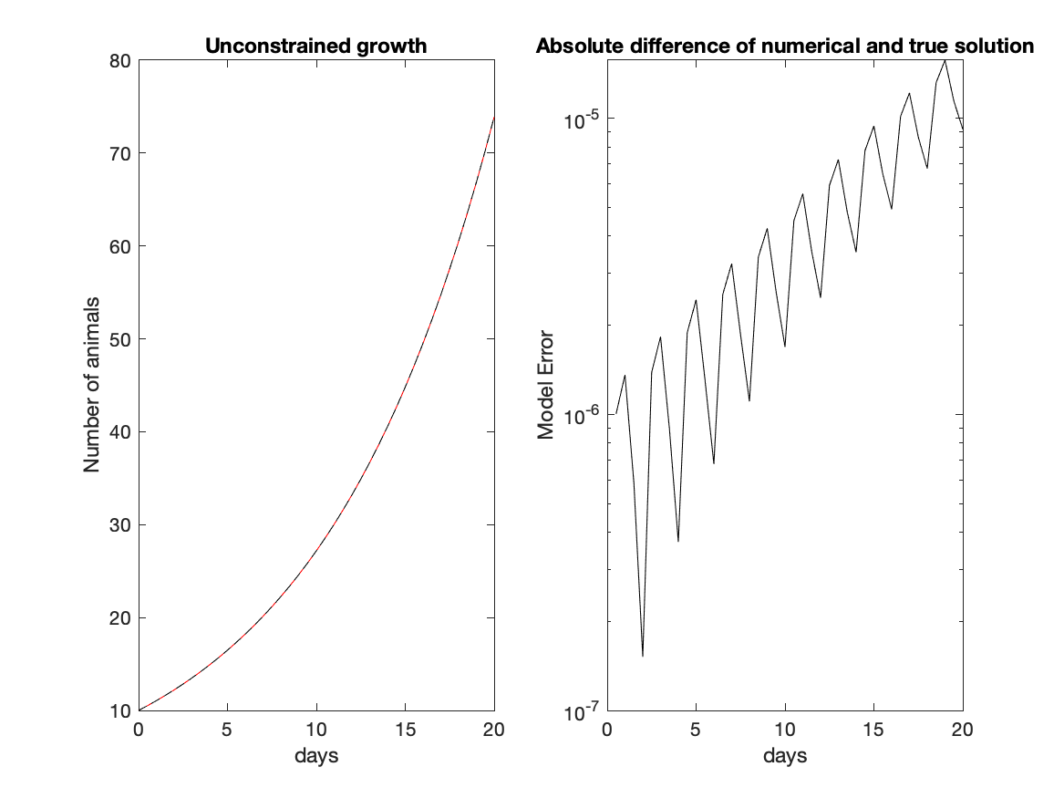
subplot(1,2,1)
plot(t,P,'r',t,TrueP,'k--')
title('Unconstrained growth')
xlabel('days')
ylabel('Number of animals')
%%% plot the absolute error for the model
subplot(1,2,2)
semilogy(t,abs(P-TrueP),'k')
title('Absolute difference of numerical and true solution')
xlabel('days')
ylabel('Model Error')
%%% save the figure
print('SS8_4c.png','-dpng')
%%% set up the RHS function
function dPdt = Malthus(t,P)
% dPdt is uncontrained growth
global g m K
%%% specify the RHS
dPdt = g * P;
%%% end function
end
True and numerical solutions (left panel) and the absolute value of the difference between true and numerical solutions (the error in the numerical solution, right panel).
From the figure below, the population grows from 10 to 50 in about 15 days. The difference between the numerical and true solution (the model error) is in the sixth or seventh decimal place of the answer.