Task: How does the behavior of the predator-prey model (below) change if the prey is controlled by a carrying capacity of 15? Write a script to solve the equations using the function PPode (below) to define the model. Use the parameter values below. Plot the solution. Comment on the change in behavior.
The ode45 solver can solve systems of coupled ODE. It is simply a matter of specifying the slope of each of the equations. Most ecosystem models track several ecosystem variables, each of which has its own dynamics.
A predator-prey ecosystem is a simple example where the prey (Prey) grow at some rate and are eaten by predators (Pred), which die at some rate. The variables (Pred, Prey) are typically number of plants or animals per area (or volume), or total weight (biomass) of each component or some such concentration. This allows the variables to be real numbers with fractional parts.
The equations for this interaction are
  d Prey/dt = g * Prey        - c * Prey * Pred
  d Pred/dt = eff * c * Prey * Pred - m * Pred
Notice that consumption of the prey by predators depends on both the number of predators and prey. There is also an efficiency factor which means that all of the prey consumed does not convert to predator biomass (numbers).
This model does not have a very interesting behavior. A more interesting model uses a carrying capacity restriction on prey growth (below).
The rate of change of both variables must be provided by the function:
function dPdt = PPode(t,P )
%  predator prey model
global g K c eff mort
dPdt=zeros(2,1);
%   prey equation
dPdt(1)=g*P(1)*(1-P(1)/K) - c*P(1)*P(2);
%   predator equation
dPdt(2)=eff*c*P(1)*P(2) - mort*P(2);
end
The script below sets the constants, which are available as global variables. The only change from the growth model in task 8.4 is that initial conditions must be provided for both prey and predators, so Po is a vector with 2 values.
The carrying capacity (K) is set to 1000 which is a prey concentration that is never reached. This choice of a large carrying capacity effectively removes any limitation of prey growth.
% PPscript
%  predator prey model
global g K c eff mort
g=1;K=1000;c=.05;
eff=.8;mort=.2;
tspan=[0 100];Po=[3 .2];
[t P]=ode45(@PPode, tspan, Po);
figure
 plot(t,P(:,1),'r',t,P(:,2),'b')
 title('prey(r) predator(b)')
 xlabel('time (day)')
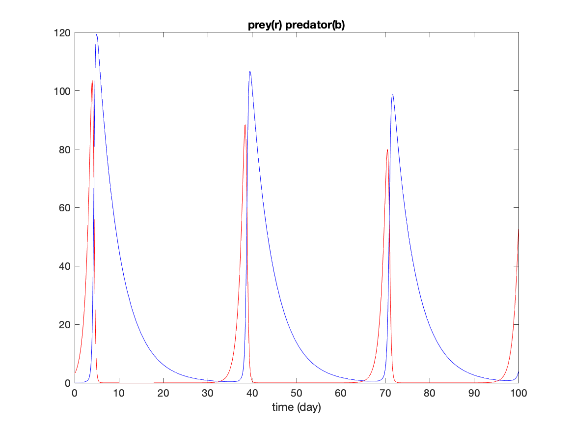
The solution shows that the prey grow quickly to a large value which is quickly eaten by the predators. Once the prey are reduced to very small levels, the predators die of starvation. Any prey preduced during this time is quickly consumed keeping prey concentration very low. Wnen the predators die to very small values, the prey are able to grow again to large concentrations which allows the predators to expand. This cycle repeats every 35 days or so.
The function ode45 returns two arrays: the first is the times (a column vector with one column), the second is a multi-column vector where the first column is variable 1, the second is variable 2 and so forth. The order of the variables is determined by the order for the rates of change in the controlling function.
At this point you can set up the solution of arbitrarily complicated ecosystem models, as long as there is no space variability. These types of models also apply to interaction of various chemical species, economics, disease transmission, among many other situations.
You can also estimate the solution of any set of coupled ODE no matter what processes are represented.
Allowing spacial variability in these models moves us to the domain of partial derivatives and partial differential equations. This is beyond the scope of this class, but it is possible to use these tools to solve spatically variable ecosystem models. I can discuss this outside of class if you are interested.
As a final comment, you can solve a higher order ODE by breaking it into a number of first order ODE. There is abundant information in the MATLAB documentationn as well as any number of web pages explaining how to do this.
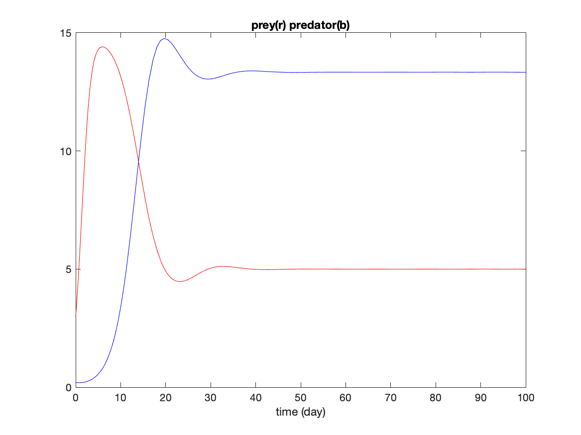
Imposing a carrying capacity of 15 on the prey, slows the growth of the prey which slows the growth of the predators. The result is that the response in both populations is smaller (smaller number of animals in the simulation). There is an initial overshoot of prey which causes an overshoot of predators, but the populations settle quickly to a steady state after about 30 days.
Flow chart to solve the task.
%%%  Define parameters for the model
%%%  set parameters for the simulation
%%%  run the simulation
%%%  plot the results
%%%    add title and legends
%%%  Define the function specifying the model
%%%    set the prey dynamics
%%%    set the predator dynamics
%%%  end the function
Script to solve the task.
% PPscript
%  predator prey model
%%%  Define parameters for the model
global g K c eff mort
g=1;K=15;c=.05;
eff=.8;mort=.2;
%%%  set parameters for the simulation
tspan=[0 100];Po=[3 .2];
%%%  run the simulation
[t P]=ode45(@PPode, tspan, Po);
%%%  plot the results
figure
 plot(t,P(:,1),'r',t,P(:,2),'b')
%%%    add title and legends
 title('prey(r) predator(b)')
 xlabel('time (day)')
%%%  Define the function specifying the model
function dPdt = PPode(t,P )
%  predator prey model
global g K c eff mort
dPdt=zeros(2,1);
%   prey equation
dPdt(1)=g*P(1)*(1-P(1)/K) - c*P(1)*P(2);
%   predator equation
dPdt(2)=eff*c*P(1)*P(2) - mort*P(2);
end%%%    set the prey dynamics
%%%    set the predator dynamics
%%%  end the function