Task: Write a script to read the global bathymetry in GlobalElev.mat. The array GlobalElev contains the elevation/depth averaged over 1 degree (lat and lon) squares. GlobalLat and GlobalLon are locations for the centers of the squares. The centers of the squares are at 0.5, 1.5, etc degrees of lon and lat. Calculate and plot the number of points in elevation and depth bins that are 1000 m wide (0-1000, 1001-2000, etc). What is the elevation/depth range over land and in the ocean with the most values? What is the average elevation for the globe including land and oceans.
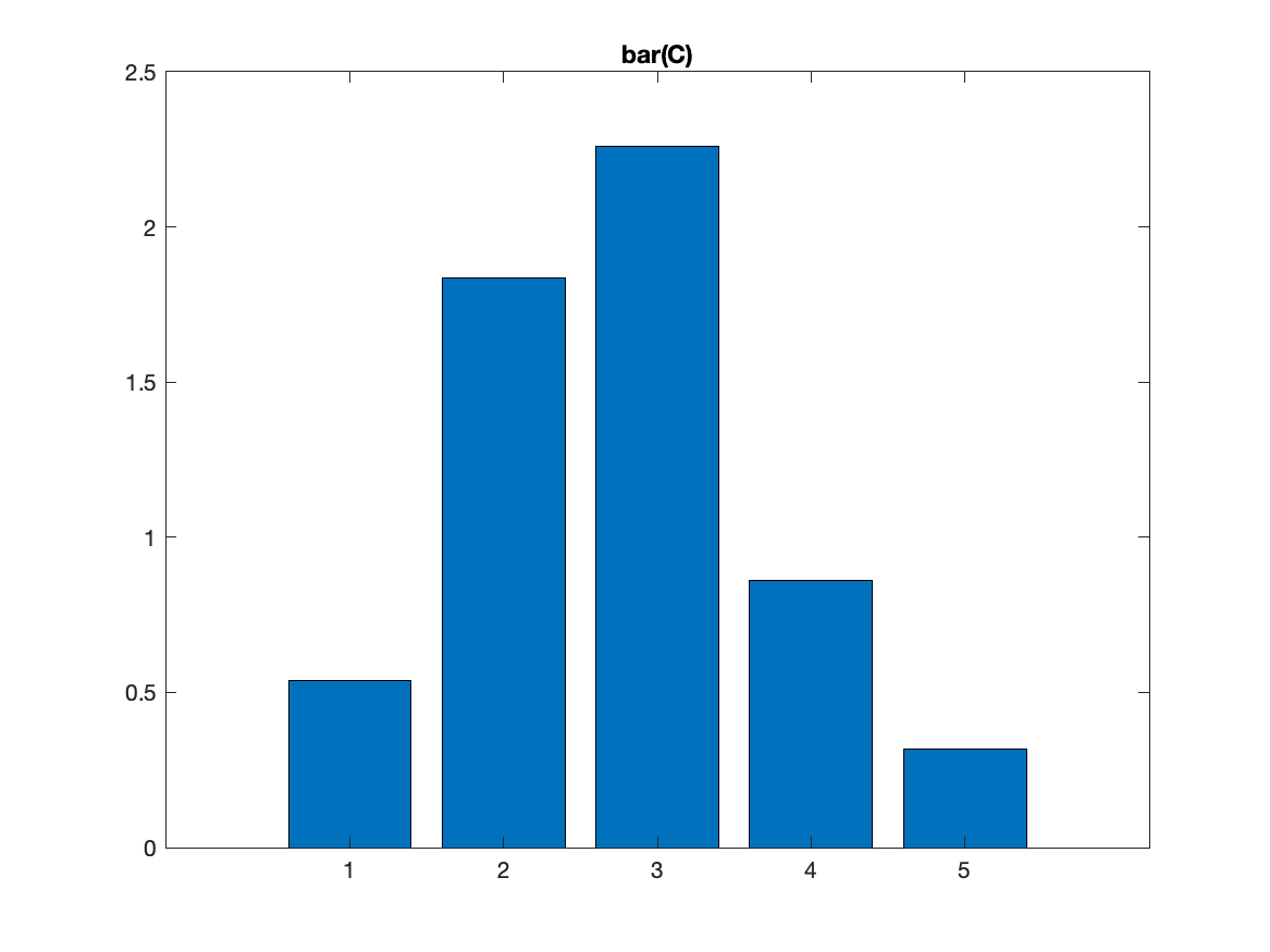
One way to display values is as a rectangular bar showing the variable values compared to zero. This can be effective for some variables, but clearly not for others. Suppose you have a list of values (C) which might be a chemical concentration at the ocean surface. Then the command bar(C); will plot the values of C as vertical bars rising from the x axis.

The command bar(x,C) plots values of C at locations x. In this case, the concentrations might be the average over a line of longitudes for a series of latitudes. Then the bar chart would show the concentration versus latitude.
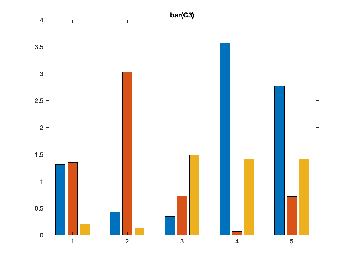
If C is a matrix, perhaps showing the concentration of several chemicals at each station (along the M rows) at several stations (along N columns), then bar(lat,C) will display clusters of M bars at N locations.

Two variations on these commands are bar3(C) and barh(C), which plot the values as 3D bars (rectangular solids) or as horizontal rectangles (extending from the y axis), respectively. Check help for these commands for more options.

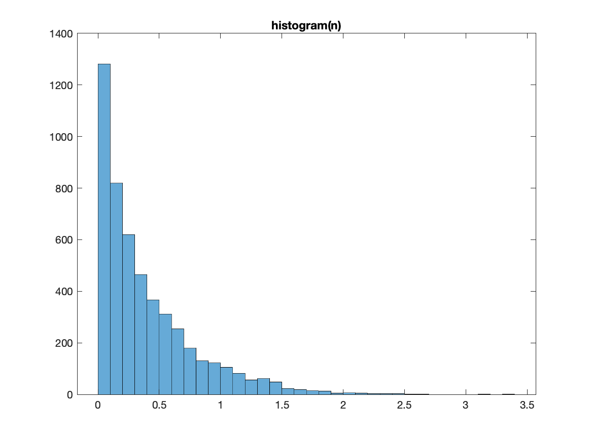
Histograms are typically displayed as bars indicating the number of values in some collection over certain ranges. This sort of plot is produced by the command histogram(x); where x is a vector or a matrix of values. This command counts the number of values in various ranges (calculated internally by default) and displays them as a bar graph.
There are a number of ways to control how the data are binned. One way is to use histogram(x,m); which requests a certain number of bins (m in this case). A more specific command is histogram(x,BE); where BE is a list of values to be used as the edges of the bins. See help for other options for histogram plot)

There are circumstances where you don't want the plot but just want the count of values in certain ranges. [C,BE]=histcounts(x); will bin the values in x, using the internally estimated bin sizes and return the count (C) in each bin defined by edges BE. For more control, [C,BE]=histcounts(x,m); request that m bins be used. It is also possible to specify the edges of the bins. See help for other options for this command.
Flow chart for the task:
%%%  read data
%%%  set edges of bins
%%%  plot histogram
%%%  add labels and title
%%%  calculate mean depth
%%%  get most common depth and elevation
Solution script for the task:
%%%  read data
  load GlobalElev.mat
%%%  set edges of bins
  DepEdge=[-8000:1000:8000];
  figure
%%%  plot histogram
  histogram(GlobalElev,DepEdge);
%%%  add labels and title
  title('Distribution of Global Elevation')
%%%  calculate mean depth
  mdepth=mean(GlobalElev,'all');
  disp(' most common elevation is 0 to 1000 m (above sea level)')
  disp(['Avg elevation is ' num2str(mdepth) ] )