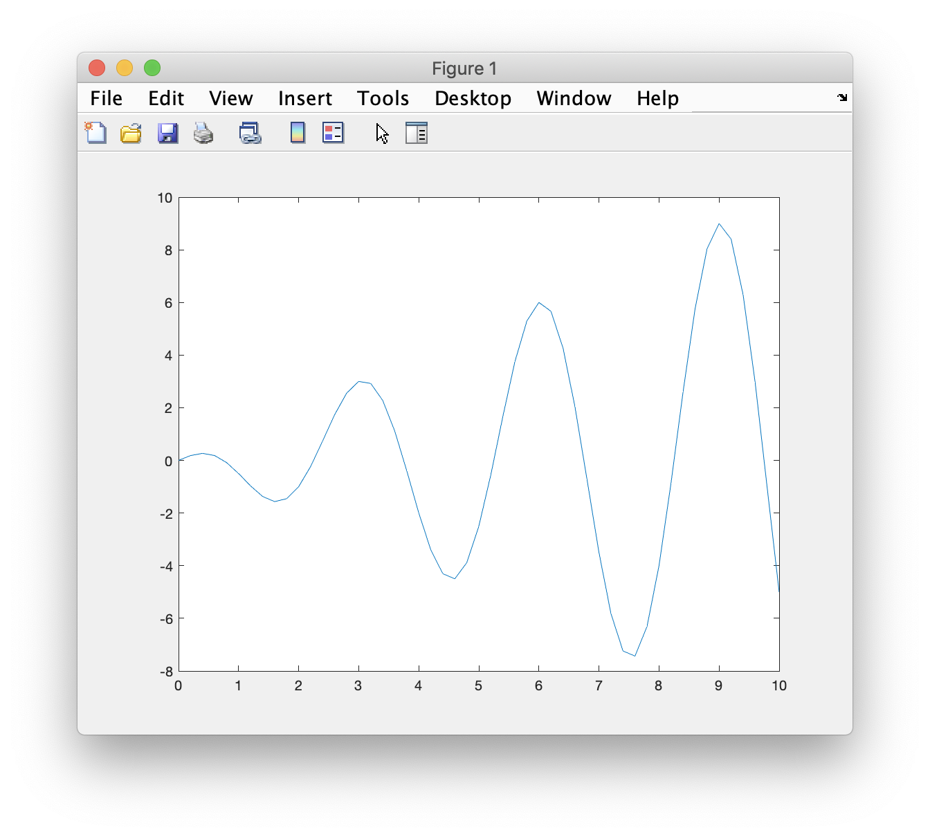
Task: In a script, define a vector (x) with values from 0 to 10 with an inteval of 0.2. Calculate values of y = x .* cos(2*pi*x/3); Make a plot of y vs x with a title and labels on the axes.
The command plot(x,y) creates a scaled plot (with a solid line) based on the values in the two arrays. It will open a graphics window (if one is not open); it will create scales for the x and y axes based on the range of values in x and y; it will put tick marks on the axes and put values on the ticks. Note that x is the horizontal axis and y is the vertical axis.
It is possible to control all of these features of the plot. Some additional controls are covered in this class but full control will wait until later when we learn how to specify options using handle graphics.
There are a number of variations on the action of this command depending on the number and type of variables passed to the command. The command plot(y) will create a plot of the values of y with the x values being the index (1 to n) of the vector. An index is a sequential counter for the values in a vector. The first value in the list has index=1 (or y(1)), the second value has index=2 (or y(2)), and so forth.
If x is a vector (a list) and y is a matrix, then plot(x,y) will plot each column of y against x. MATLAB will choose colors for the different lines based on the current color map (which we will learn about later).
As a general rule, MATLAB works on values in columns in multi-dimensional arrays. We will see how to take advantage of this in the coming tasks.
You can control the line type and color with options to the plot command which we will see shortly.
The commmand title('Title') will put the string at the top center of the graph. Similarly, the commands xlabel('X Label') and ylabel('Y Label') will put the text you want at the bottom center and left center of the plot, respectively. These commands put labels on the x and y axes of the plot.

The argument of these commands can be any character string that you want. An interesting option is to create a variable with the string that you want to use. So you could do the following:
  TitleText='Daily Temperature';
  xText='Time(day)';
  yText='degree C';
  title(TitleText)
  xlabel(xText)
  ylabel(yText)
This programming idea would be useful for the creation of a series of plots with the same general content.
It is possible to put special characters in the character strings using LaTeX characters. For example, the greek characters "mu", "theta", and "rho" are indicated by \mu, \theta, and \rho, respectively.
Subscripts and superscripts are indicated with _ and ^. So the string 'km^2' would put a 2 superscript indicating square kilometers. The string 'CO_2' would create the familiar chemical symbol for carbon dioxide.
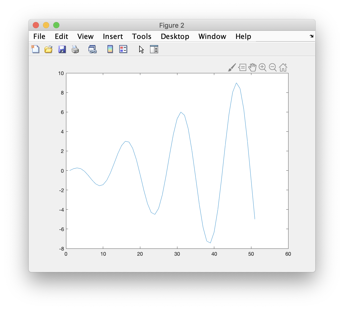
In all of the previous graphics commands, there has been one graphics window open. Every new use of the command plot erased the previous plot and created a new one. You can force the creation of a new graphics window with the command figure. The following sequence will open a new graphics window and produce a line plot.
figure
plot(x,y)
title('New Plot')
Note that if there is an graphics window open, it will not be erased or
changed. It this way, you can create a number of graphs, each in its
own graphics window.
Each graphics window has an identifying number so it is possible to refer to earlier windows. Or, you can designate the identifier for a new window by adding a number to the command: figure(1). If the window already exists, then it is the focus (or recipient) of the next graphics commands. For example, consider the following commands:
figure(1)
plot(x1,y1)
figure(2)
plot(x2,y2)
figure(1)
title('First Plot')
figure(2)
title('Second Plot')
figure(1)
xlabel('time(days)')
figure(2)
xlabel('distance(km)')
%  and so on...
These create two different graphs by alternately adding commands to two
different graphics windows. Clearly, this is not a recommended way
to create multiple plots, but you might find circumstances where you
need to work on more than one graphics window.
Script to complete this task:
% task31.m
 x=0:.2:10;
 y= x.* cos(2*pi*x/3);
 figure
 plot(x,y)
 title('Class 3 plot')
 xlabel('distance')
 ylabel('elevation')