Task: Write a script to read the data file below. Extract the variables time and D3. Calculate the mean and variance of D3. Plot D3 vs time. Add a line on the plot showing the mean value. Add two other lines (in different colors) showing the mean plus and minus the standard deviation. Add appropriate labels and a title.
Use the data file fitdata.dat for the exercises in this class. The file has four data columns with time in the first column and associated data in the other three columns. Refer to values as D1, D2 and D3 for later convenience.
We have already seen a way to calculate the mean of a variable using two functions: sum and length. There is a MATLAB function, mean, that does the calculation in one step: meanD1=mean(D1);.
There is another statistical quantity, mode, which is another way to represent the central tendency of a set of numbers. It is defined to be the middle value of a list of numbers organized from smallest to largest. For numbers that are normally distributed, the mean and the mode are the same. In a set of numbers with outliers (values distinctly different from the rest of the values), the mode is a better representation of the central value. There are tools in MATLAB to sort a set of numbers, it is easier to use the MATLAB function mode for the calculation.
The variance of a set of numbers is a measure of the variability of the numbers around the mean. Specifically, the variance is defined as the average of the square of the deviation of the values from their mean:
  meanD1=mean(D1);
  vD1=D1-meanD1;
  varD1=sum(vD1.^2)/length(D1);
% varD1=var(D1);   % a direct calculation
The last line provides a direct way to calculate the variance of a list of numbers.
You should notice that the variance will have units that are the square of the units of thte original data. If D1 is a set of temperatures in degree C, then varD1 has units of (degree C)^2. In order to compare this measure of variability with the original data, we need to take the square root of the variance.
The standard deviation is defined to be the square root of the variance. The variability of a set of numbers is represented as the mean plus and minus the standard deviation. The standard deviation can be calculated as:
 varD1=var(D1);
 stdD1=sqrt(varD1);
% stdD1=std(D1);  % a direct calculation
The last line gives a direct way to calculate the standard deviation.
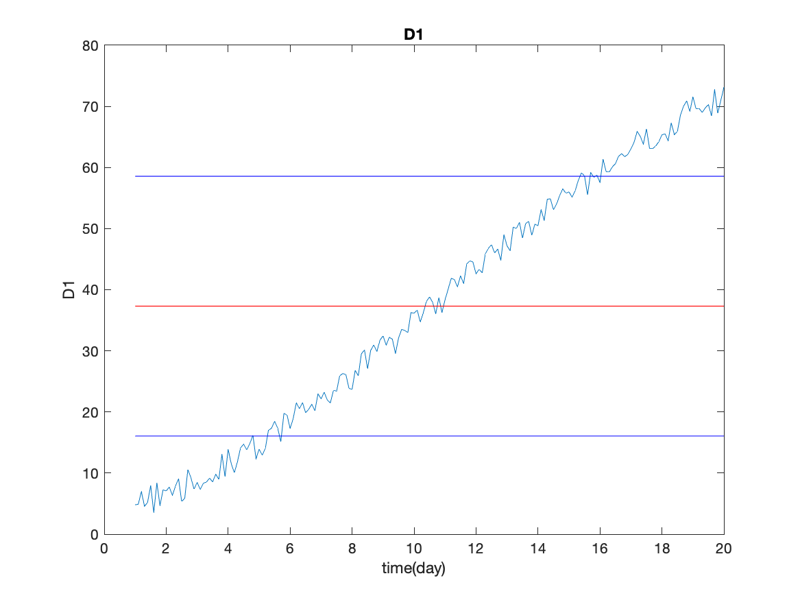
Here is the figure showing the mean and standard deviation of the third data column.
In some discussions of statistics, the variance is defined as varD1=sum(vD1.^2)/(length(D1)-1); where the sum is divided by one less than the number of values in the sum. The explanation is that the sum of the squared deviations is divided by the degrees of freedom (df) in the sum, which is one less than the total number of values in the original data. The original data has df equal to the total number of independent values in the data set. Calculating the mean (the first moment of the data) uses one degree of freedom, so the variance (second moment) has one fewer degrees of freedom. In practical terms, for most environmental data sets, the difference in the result is insignificant whether dividing by length(D1) or (length(D1)-1).
One additional comment: the divisor should be the number of independent values in the data set. Successive environmental measurements are rarely independent so the df is frequently less (sometimes much less) than the number of values in a data set. For example, think of hourly measurements of surface water temperature in Chesapeake Bay. Will you get better statistics by measuring the temperature every minute? It gives 60 times the number of values but do all of these extra numbers better constrain temperature mean or variance for a given month? Resolving this issue is outside of the scope of this class.
As a final comment, we saw in the last class that if the data have missing values represented by NaN, then these values must be removed from the data list before calculating statistics. While we found an easy way to do this in the previous class, there are MATLAB functions nanmean, nanvar, and nanstd which do the indicated calculations removing any NaN values from the lists before calculating the indicated statistics.
Flow chart for this task.
%%%  task51.m
%%%  read data, extract variables
%%%  calculate mean and standard dev
%%%  plot D3
%%%  add lines for mean, mean +- std
%%%  add legends and a title
Here is the script to generate the answer to this task.
%%%  task51.m
%%%  read data, extract variables
  data=load('fitdata.dat');
  time=data(:,1);D3=data(:,4);
%%%  calculate mean and standard dev
  mD3=mean(D3);sD3=std(D3);
%%%  plot D3
  figure
    plot(time,D3)
%%%  add lines for mean, mean +- std
    hold on
    plot([time(1) time(end)],[mD3 mD3],'r')
    plot([time(1) time(end)],[mD3-sD3 mD3-sD3],'b')
    plot([time(1) time(end)],[mD3+sD3 mD3+sD3],'b')
    hold off
%%%  add legends and a title
    title('D3')
    xlabel('time (day)')
    ylabel('D3')