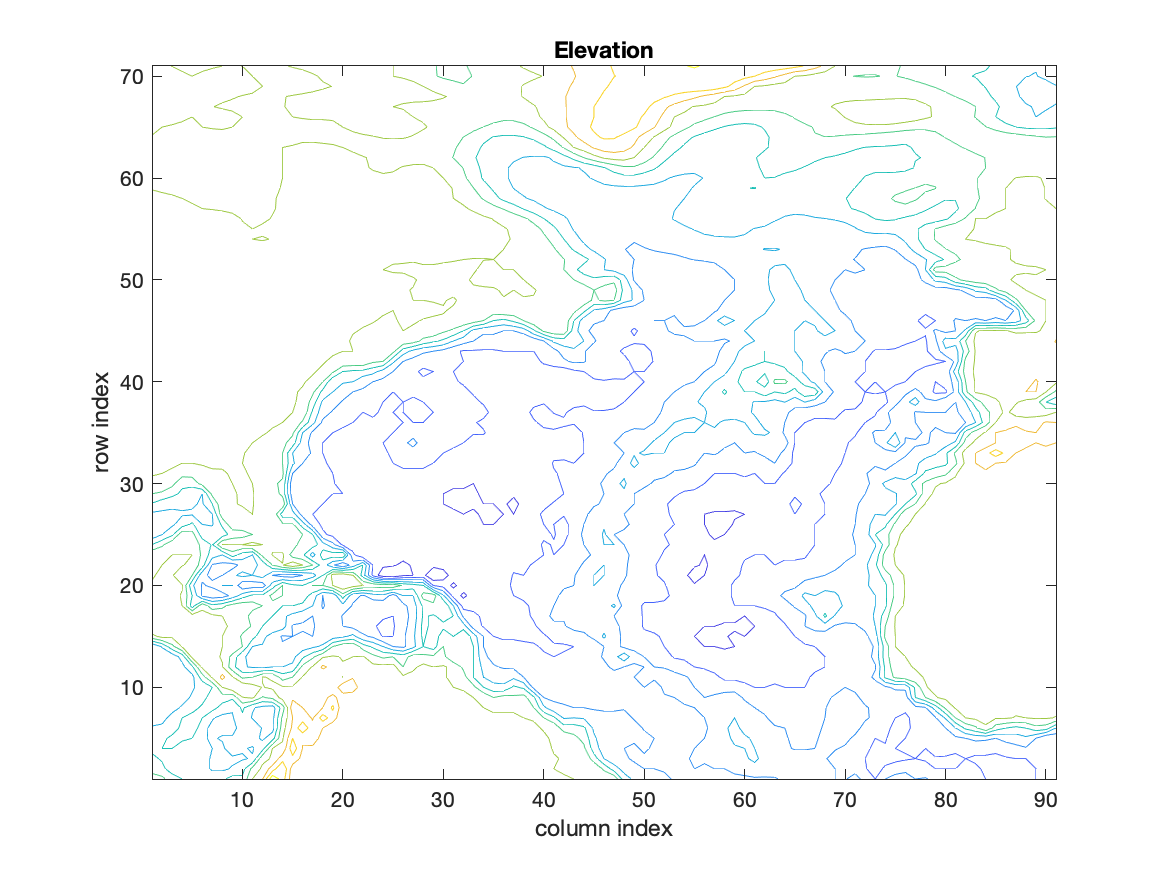
Task: Create a topographic map of the North Atlantic Ocean and surrounding land. The elevation data (digital elevation map (DEM) in units of m) are provided every degree of latitude and longitude in NAbathy.mat. Positive elevation is above mean sea level, negative is below. Use load to read the file which contains a 2D array (NAelev) and two 1D arrays (NAlat and NAlon). Note that longitude is 0 to 360 degrees.
There are many times when environmental data is given as values at locations on a surface. For example, we might have values of ocean surface temperature or elevation of the surface of the earth at locations given by latitude and longitude. We would like to display this information by estimating lines on the surface that follow locations of constant values (isolines).
In other circumstances, we might have measurements with depth at a number of locations in the ocean (or on the earth). We would like to show values in the vertical plane where the measurements are the same by drawing isolines. This is a vertical plane or section plot.
We might want to see the value of some function that depends on two variables. This might be a plot of ocean water density as a function of temperature and salinity. It might be growth rate of a phytoplankton as a function of temperature and light intensity. There are many other possible uses for such 2D displays.
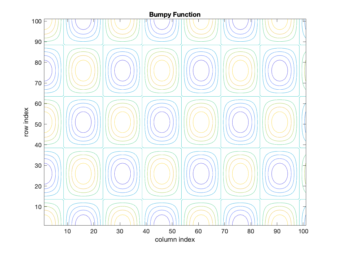
MATLAB has a number of graphics tools to display values on a 2D surface. The easiest is a contour plot; the simplest form is
  x=0:.1:10;y=0:.1:10;
  nx=length(x);ny=length(y);
  F=zeros(ny,nx);
  for ix=1:nx
     for iy=1:ny
       F(iy,ix)=cos(2*pi*x(ix)/3).*cos(2*pi*y(iy)/5);
     end
  end
  figure
  contour(F)
  title('Bumpy Function')
  xlabel('column index')
  ylabel('row index')
The commands to
label the figure (title, xlabel, ylabel)
are the same as we saw before with simple line drawings.
By default, the command will look at the range of values in the array F and choose ten or so values for the contour lines.
The command assumes that the values in the array F are arranged in an orderly fashion. It assumes that the value F(1,1) is at the origin of the surface and the values along columns are located at increasing values of x. The values in increasing rows are increasingly towards increasing y.
The command above only presented the values in the array with no indication of the location of the points on the surface. The contour command uses the array indexes as locations. It also assumes that the values are separated by uniform space intervals.
The contoured field has the appearance of a topographic map, where lines show uniform values of F.
The flow chart for the task solution:
%%%  load data
%%%  contour data
Script to solve the task:
%%%  load data
load('NAbathy.mat'); %  get variables NAelev, NAlat, NAlon
%%%  contour data
figure
  contour(NAelev)
  title('North Atlantic Elevation (m)')
  xlabel('column index')
  ylabel('row index')
The resulting image will look like