Task: Add geophysical locations (latitude and longitude) to the bathymetry map from the first task in this class to create a true topographic map. Use the NAbathy.mat data.
The contours created in the tasks 9.1 and 9.2 were interesting but there is no way to locate the points on this map because there were no position indicators (other than array index values which are not helpful).
The contouring program needs the location of the individual points being contoured. The program uses two additional arguments indicating locations (x, y) for the values being contoured.
Before continuing with the North Atlantic example, consider a simpler situation where a function of two variables is created. Suppose you want to represent a mountain by a 2D gaussian function which depends on two locations (x,y), where each variable is a list of locations. The idea is that h(x,y) = h(x(i),y(j)) = h(i,j). The first part of this statement is that there is a function (h) that depends on a location specified by two values (x,y). The second part is that there are a list of discrete locations (x(i), y(j)) where the locations are in lists of numbers. The final part is a matrix of values (h(i,j)) which is the value of the function at the location indicated by the indexes (i,j).
Although it is easy to evaluate the function as stated, it is easier to use locations for every point (i,j) so that X(i,j) and Y(i,j) are locations for every point in the matrix of values (h(i,j)). In this case, h(i,j)=h(X(i,j),Y(i,j)).
The simplest situation is that every row of X has the same locations and every column of Y has the same location. This is easy to create in MATLAB with the function meshgrid().
meshgrid produces 2D arrays of locations to evaluate the function. Specifically, [X Y]=meshgrid(x,y) takes the two input lists (x,y) to create the 2D arrays (X,Y). This is done by taking each row of x values and copying them enough time to create enough rows to match the length of y. Similarly, y is a column of values which is copied into enough columns to match the length of x.
As a simple example, let x=(1 2 3) and y=(6,7,8,9). Then [X Y]=meshgrid(x,y) creates arrays
   X = [ 1 2 3]
       [ 1 2 3]
       [ 1 2 3]
       [ 1 2 3]
and
Y = [9 9 9]
    [8 8 8]
    [7 7 7]
    [6 6 6]
In this way, each location in the 2D grid of points is located by arrays X(i,j) and Y(i,j)
Consider the following script.
%   2D gaussian mound
%
xo=25; yo=40;  % (km)  location of peak of mound
wx=10;wy=50;   % (km) width scale for the mound
ho = 2000;     % (m)  height of peak of mound
x=-100:2:200;y=-100:2:200;  % (km)  horizontal domain
[X Y]=meshgrid(x,y);
h= ho*exp(-((X-xo).^2/(2*wx.^2))-((Y-yo).^2/(2*wy.^2)));
figure
  [con han]=contour(X,Y,h);
  clabel(con,han)
In the North Atlantic data file, there are arrays NAlat and NAlon indicating the latitude and longitude of the array points. However, the contouring program wants a location for every value in the input array.
Then meshgrid which takes the two vectors and converts them into arrays. The elevation array, NAelev, is a 2D array. The columns are located at longitudes indicated by NAlon and the rows are located at latitudes indicated by NAlat.
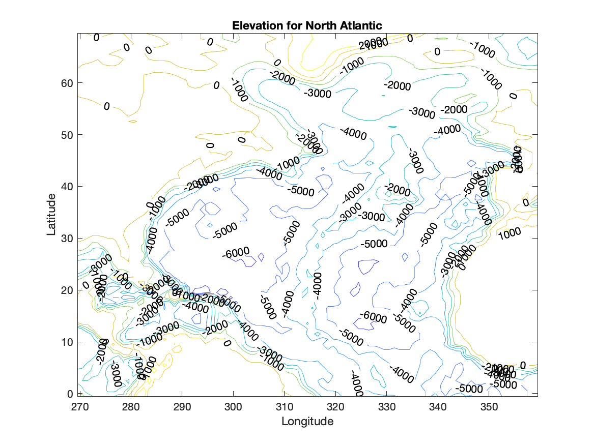
The script below creates the location arrays for the elevation points and contours the elevation with the axis labels in degrees of longitude and latitude.
   [LonArray LatArray]=meshgrid(NAlon,NAlat);
   figure
   [con han]=contour(LonArray,LatArray,NAelev,[-7000:1000:2000]);
   clabel(con,han)
   xlabel('Longitude')
   ylabel('Latitude')
   title('Elevation for North Atlantic')
The meshgrid function gets the size of the2D arrays from the sizes of the first and second arguments; let them be nx and ny, to be specific. Then it creates two ny by nx arrays. It copies NAlon into all ny rows of LonArray and it copies NAlat into all nx columns of LatArray. In this way, each point in NAelev has an associated latitude and longitude.
Recent versions of MATLAB allow the use of 1D arrays (NAlon,NAlat) as arguments to these 2D plotting routines. They will internally create the appropriate 2D location arrays and give the expected plot. Older versions of MATLAB will report an error if 1D location arrays are used.
The flow chart for the task solution:
%%%  load data
%%%  create location arrays
%%%  choose contour intervals
%%%  contour data
%%%  label contour lines
%%%  add title and labels
Script to solve the task:
%%%  load data
load('NAbathy.mat'); %  get variables NAelev, NAlat, NAlon
%%%  create location arrays
[LonArray LatArray]=meshgrid(NAlon,NAlat);
%%%  choose contour intervals
ci=[-7000:1000:2000];
%%%  contour data
figure
  [C H]=contour(LonArray,LatArray,NAelev,ci);
%%%  label contour lines
  clabel(C,H);
%%%  add title and labels
  title('North Atlantic Elevation (m)')
  xlabel('column index')
  ylabel('row index')