Task: Use the North Atlantic elevation data (details in task 9.1 ) to create a perspective plot with surf. Use view to look at the graph from the south elevated above mean sea level. Use meshgrid to create location arrays for the points. Add labels on x and y axes so you can identify latitude and longitude.
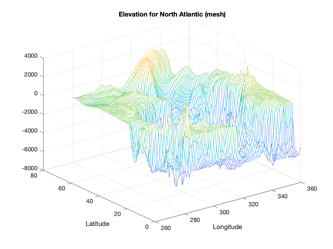
The command mesh(xA,yA,E) represents the array of numbers, E as elevations, located at positions (xA,yA). Specifically, it creates a set of boxes with the corners at the locations (xA,yA) and elevated according the values of E.
   mesh(LonArray,LatArray,NAelev)
   xlabel('Longitude')
   ylabel('Latitude')
   title('Elevation for North Atlantic (mesh)')
What results is a mesh of lines that represent the shape of E as if it were elevations. The mesh of lines is colored in proportion to values of E. For the standard color map, the larger values of E will be red while the smaller values will be blue with proportional color changes between.
A similar command surf(xA,yA,E) creates a mesh of points at locations (xA,yA) using E as an elevation. However, surf colors in the mesh to create a solid looking multicolor surface.
   surf(LonArray,LatArray,NAelev)
   xlabel('Longitude')
   ylabel('Latitude')
   title('Elevation for North Atlantic (surf)')
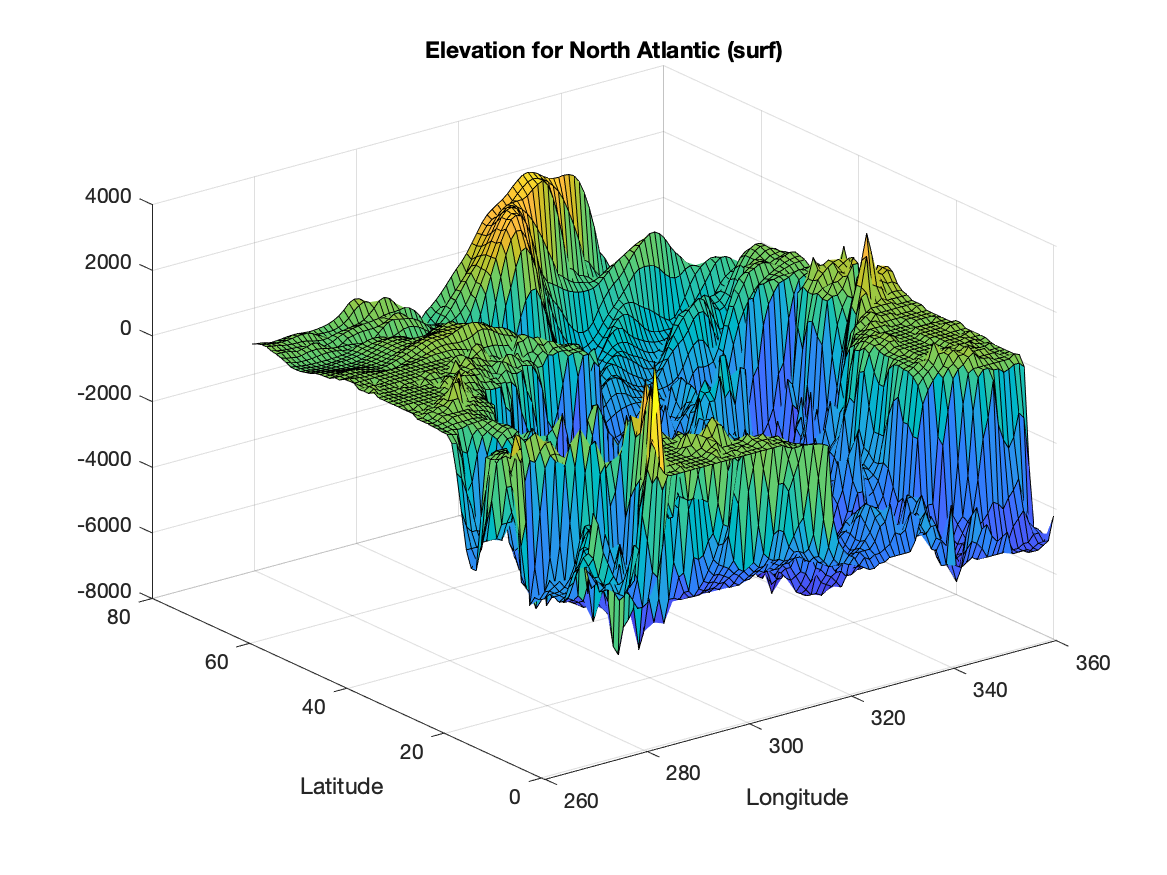
By default, the image has black lines showing the locations of the patches and the colors across the patch are proportional to the average of the elevation at the corners.
The color representation can be controlled by shading which has three choices: FLAT, INTERP and FACETED.
FACETED uses a constant color proportional to the E value of the corner nearest to the origin (smallest indexes). This choice also adds black lines along the edges of the patches. This is the default.
FLAT is the same as FACETED, except that the black lines are not included.
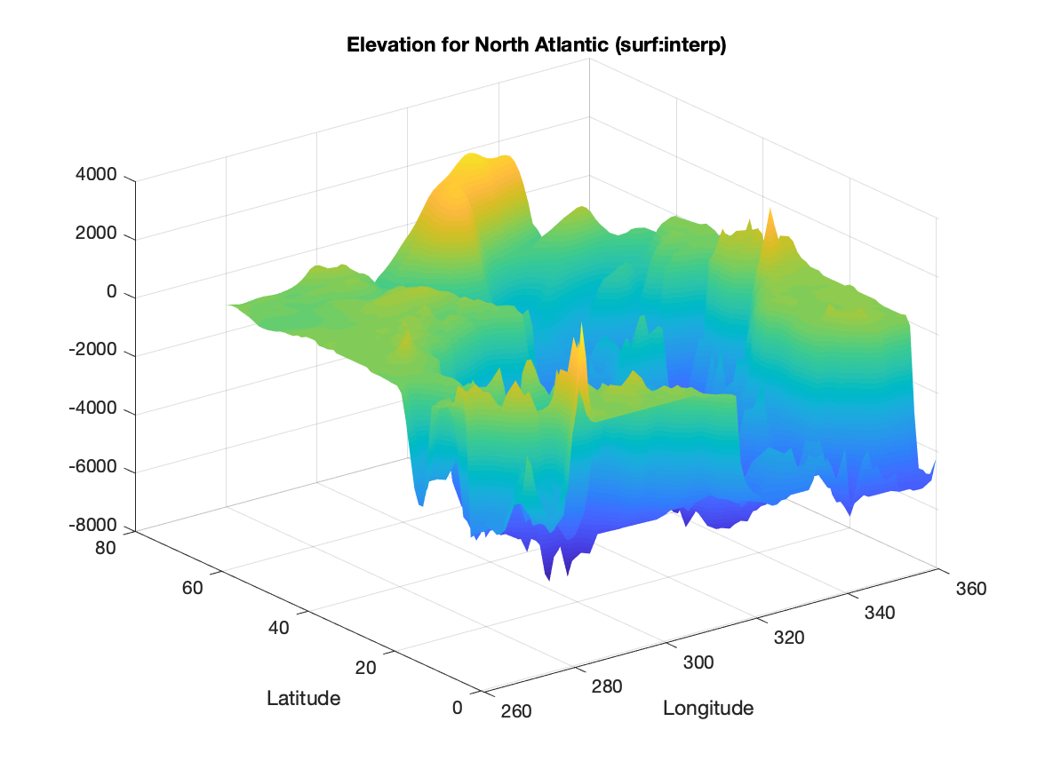
INTERP smoothly varies the color across each patch in proportion to the E values at the corners. This choice give the appearance of a smoothly varying color over the whole surface.
   surf(LonArray,LatArray,NAelev)
   xlabel('Longitude')
   ylabel('Latitude')
   title('Elevation for North Atlantic (surf:interp)')
   shading interp
It is possible to control the viewpoint of these 3D surface with view(AZ,EL), where the input arguments are azimuth (AZ) and elevation (EL). Both of the input arguments are angles in degrees. In all cases, the view is through the center of the plot.
Positive azimuth is measured counterclockwise while negative are clockwise. AZ=0 means looking from somewhere in negative y through the origin along the y axis. The default value of AZ is -37.5 degrees (looking through the origin towards the northeast).
Positive elevation is measured above x-y plane, while negative is below the x-y plane. The default elevation is 30 degrees.
   surf(LonArray,LatArray,NAelev)
   xlabel('Longitude')
   ylabel('Latitude')
   title('Elevation for North Atlantic (surf:view)')
   view(30,30)
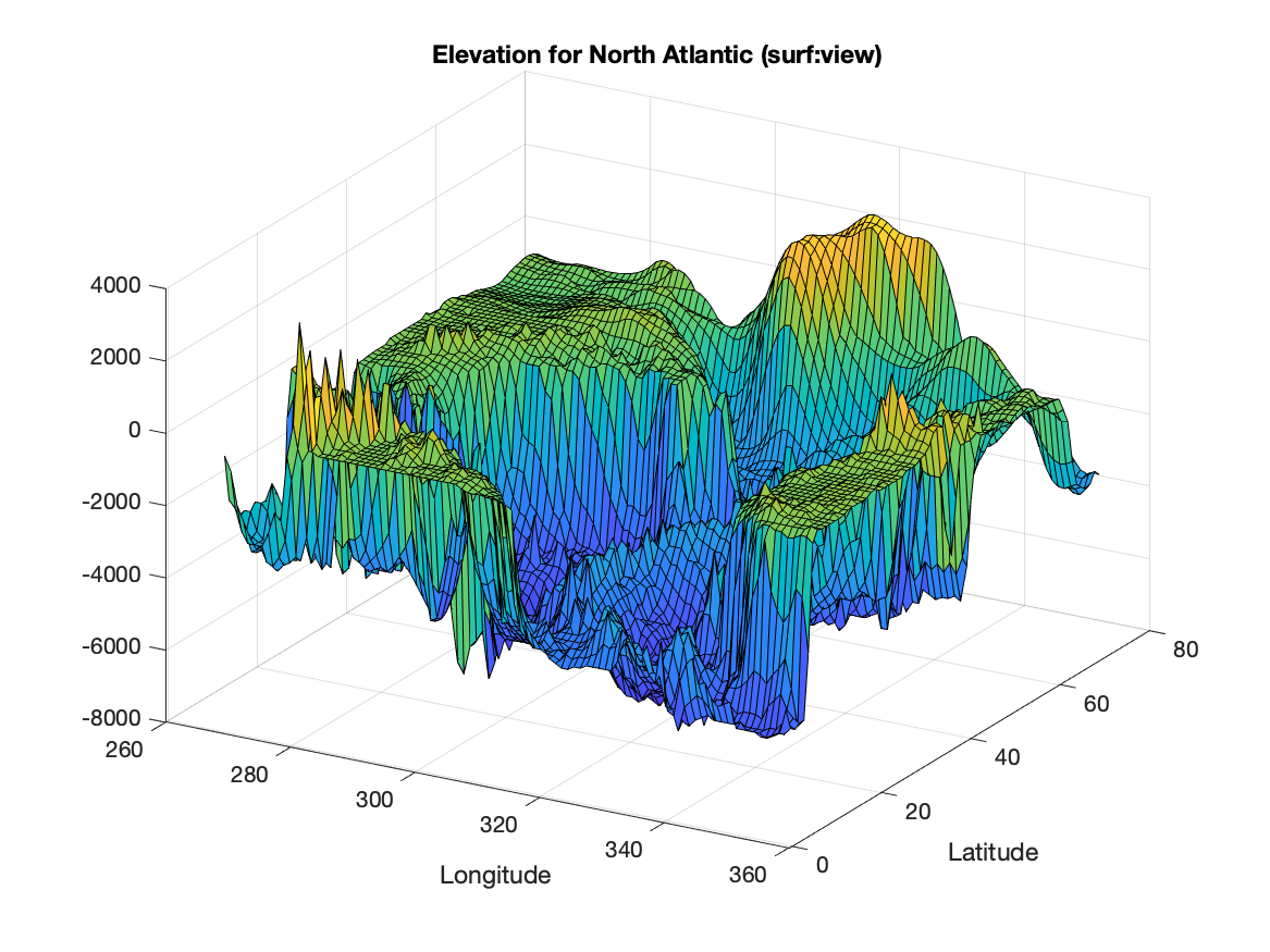
Choosing view(0,90) is essentially looking down from directly overhead.
The flow chart for the task solution:
%%%  load data
%%%  create location arrays
%%%  display data with surf
%%%  set viewpoint to be from the south and up 30 degrees.
%%%  add title and labels
Script to solve the task:
%%%  load data
load('NAbathy.mat'); %  get variables NAelev, NAlat, NAlon
%%%  create location arrays
[LonArray LatArray]=meshgrid(NAlon,NAlat);
%%%  display data with surf
figure
  surf(LonArray,LatArray,NAelev);
%%%  set viewpoint
  view(0,30)
%%%  add title and labels
  title('North Atlantic Elevation (m)')
  xlabel('column index')
  ylabel('row index')