Task: Convert a set of measurements at random points to a gridded set of measurements. Use a basic functional structure of F(x,y) = sin(pi*x).*sin(pi*y), for x and y in the range [0 1]. Choose a set of N=100 random points in the domain with xd=rand(N,1) and yd=rand(N,1). Evaluate the function Fd=sin(pi*xd).*sin(pi*yd). Grid these random values onto a regular (x,y) grid with a spacing of 0.02. Refine the gridded values in the center of the domain with a spacing of 0.01 for x, y between 0.4 and 0.6. Use contour to plot the true, recovered and refined fields.
There are two tools for interpolation in 2D: interp2 and griddata. It turns out that these can interpolate in 3D and higher dimensions, but you can discover these aspects of these tools, after working with 2D arrays.
Suppose you have a regular array of points in 2D at which you have values. To be specific, the points are located at a regular array of points xd and yd which are 1D arrays. Then the data values (V) are located at points defined by [X Y]=meshgrid(xd,yd);.
You can interpolate these values to a different set of points (xi,yi) which form a rectangular array [Xi Yi]=meshgrid(xi,yi);.
Be aware that all of the (xi,yi) points must be inside the values defined by (xd,yd). Otherwise, the interpolated values will be NaN.
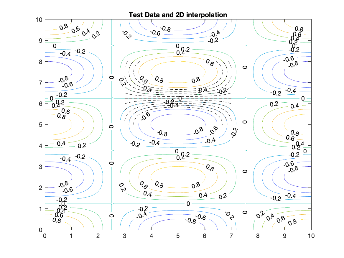
This procedure is illustrated in the following way which generates a smooth set of test data. The interpolation creates a set of data on a finer grid at the center of the test data. The interpolated data is contoured with half of the contour interval as the test data so a comparison is possible.
  xd=0:.1:10;yd=0:.1:10;
  [XD YD]=meshgrid(xd,yd);
  Fd=cos(pi*XD/5).*cos(2*pi*YD/5);
  xi=4:.05:6;yi=4:.05:6;
  [Xi Yi]=meshgrid(xi,yi);
  Fi=interp2(XD,YD,Fd,Xi,Yi);
  figure
   [con han]=contour(XD,YD,Fd,[-1:.2:1]);
   clabel(con,han);
   title('Test Data and 2D interpolation')
   hold on
   contour(Xi,Yi,Fi,[-.5:.1:.5]);
   hold off
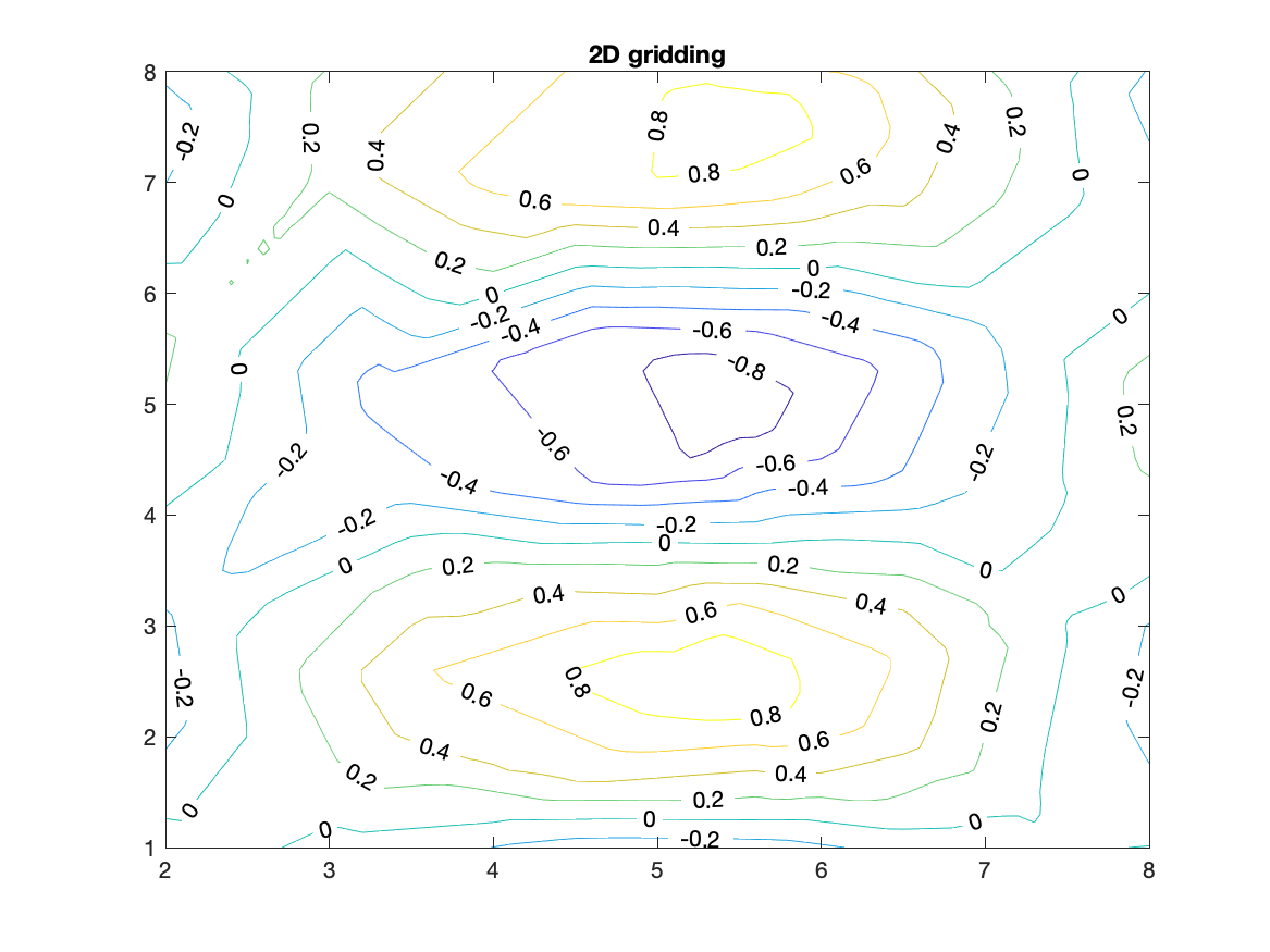
A more difficult problem is to take values at scattered points and convert them to a regular grid of values. This problem is common in environmental sciences since we cannot always control where we make measurements. The tool to use is griddata.
Setup of the problem with a set of values (Fs) at locations (xs,ys), which are scattered over some area. Note that all three of these arrays are 1D. The function call is Fi=griddata(xs,ys,Fs,Xi,Yi); where (Xi,Yi) are a regular grid of locations defined above with meshgrid.
An example of the use of this function is
%  create a random set of observation points
  N=200;xs=10*rand(N,1);ys=10*rand(N,1);
%    calculate the test  function at the observation points
  Fs=cos(pi*xs/5).*cos(2*pi*ys/5);
  xi=2:.1:8;yi=1:.1:8;   % interpolation points
  [Xi Yi]=meshgrid(xi,yi);
  Fi=griddata(xs,ys,Fs,Xi,Yi);
  figure
   [con han]=contour(Xi,Yi,Fi);
   clabel(con,han);
   title('2D gridding')
Notice that this figure compares reasonably well to the center part of the previous figure. So, it is possible to reconstruct the large scale structure of a set of measurements with a relatively small number of values, as long as they are scattered more or less uninformly over the area of interest.
As an exercise, you might try the task above with different numbers of data points, or with a data function with more structure to see how many points are required to recover a function.
Flow chart to solve the task:
%%%  set up true field
%%%  plot true field
%%%  add labels and titles
%%%  choose random x,y points
%%%  evaluate the test function at these points
%%%  create a regular grid of values from these random points
%%%  plot the recovered field
%%%  add labels and titles
%%%  refine the gridded values near the center of the grid
%%%  plot refined field<
%%%  add labels and titles
Script to solve the task:
%%%  set up true field
x=0:.02:1;y=0:.02:1;
[xA yA]=meshgrid(x,y);
F=sin(pi*xA).*sin(pi*yA);
%%%  plot true field
figure
 [con han]=contour(xA,yA,F);
  clabel(con,han);
%%%  add labels and titles
 title('True Field')
%%%  choose random x,y points
N=100;xd=rand(N,1);yd=rand(N,1);
%%%  evaluate the test function at these points
Fd=sin(pi*xd).*sin(pi*yd);
%%%  create a regular grid of values from these random points
Fi=griddata(xd,yd,Fd,xA,yA);
%%%  plot recovered field
figure
 [con han]=contour(xA,yA,Fi);
  clabel(con,han);
%%%  add labels and titles
 title('Recovered Field')
%%%  refine the gridded values near the center of the grid
xi=0.4:.01:0.6;yi=0.4:.01:0.6;[xiA yiA]=meshgrid(xi,yi);
Fi2=interp2(xA,yA,Fi,xiA,yiA);
%%%  plot refined field
figure
 [con han]=contour(xiA,yiA,Fi2);
  clabel(con,han);
%%%  add labels and titles
 title('Refined Field')